Trajectory Optimization and Control of Flying Robot Using Nonlinear MPC

This example shows how to find the optimal trajectory that brings a flying robot from one location to another with minimum fuel cost using a nonlinear MPC controller. In addition, another nonlinear MPC controller, along with an extended Kalman filter, drives the robot along the optimal trajectory in closed-loop simulation.

Flying Robot

The flying robot in this example has four thrusters to move it around in a 2-D space. The model has six states:

• x(1) - x inertial coordinate of center of mass

• x(2) - y inertial coordinate of center of mass

• x(3) - theta, robot (thrust) direction

• x(4) - vx, velocity of x

• x(5) - vy, velocity of y

• x(6) - omega, angular velocity of theta

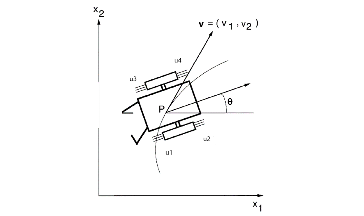
For more information on the flying robot, see [1]. The model in the paper uses two thrusts ranging from -1 to 1. However, this example assumes that there are four physical thrusts in the robot, ranging from 0 to 1, to achieve the same control freedom.

Trajectory Planning

The robot initially rests at [-10,-10] with an orientation angle of pi/2 radians (facing north). The flying maneuver for this example is to move and park the robot at the final location [0,0] with an angle of 0 radians (facing east) in 12 seconds. The goal is to find the optimal path such that the total amount of fuel consumed by the thrusters during the maneuver is minimized.

Nonlinear MPC is an ideal tool for trajectory planning problems because it solves an open-loop constrained nonlinear optimization problem given the current plant states. With the availability of a nonlinear dynamic model, MPC can make more accurate decisions.

In this example, the target prediction time is 12 seconds. Therefore, specify a sample time of 0.4 seconds and prediction horizon of 30 steps. Create a multistage nonlinear MPC object with 6 states and 4 inputs. By default, all the inputs are manipulated variables (MVs).

Ts = 0.4;
p = 30;
nx = 6;
nu = 4;
nlobj = nlmpcMultistage(p,nx,nu);
nlobj.Ts = Ts;

For a path planning problem, it is typical to allow MPC to have free moves at each prediction step, which provides the maximum number of decision variables for the optimization problem. Since planning usually runs at a much slower sampling rate than a feedback controller, the extra computation load introduced by a larger optimization problem can be accepted.

Specify the prediction model state function using the function name. You can also specify functions using a function handle. For details on the state function, open FlyingRobotStateFcn.m. For more information on specifying the prediction model, see Specify Prediction Model for Nonlinear MPC.

nlobj.Model.StateFcn = "FlyingRobotStateFcn";

Specify the Jacobian of the state function using a function handle. It is best practice to provide an analytical Jacobian for the prediction model. Doing so significantly improves simulation efficiency. For details on the Jacobian function, open FlyingRobotStateJacobianFcn.m.

nlobj.Model.StateJacFcn = @FlyingRobotStateJacobianFcn;

A trajectory planning problem usually involves a nonlinear cost function, which can be used to find the shortest distance, the maximal profit, or as in this case, the minimal fuel consumption. Because the thrust value is a direct indicator of fuel consumption, compute the fuel cost as the sum of the thrust values at each prediction step from stage 1 to stage p. Specify this cost function using a named function. For more information on specifying cost functions, see Specify Cost Function for Nonlinear MPC.

for ct = 1:p
    nlobj.Stages(ct).CostFcn = 'FlyingRobotCostFcn';
end

The goal of the maneuver is to park the robot at [0,0] with an angle of 0 radians at the 12th second. Specify this goal as the terminal state constraint, where every position and velocity state at the last prediction step (stage p+1) should be zero. For more information on specifying constraint functions, see Specify Constraints for Nonlinear MPC.

nlobj.Model.TerminalState = zeros(6,1);

It is best practice to provide analytical Jacobian functions for your stage cost and constraint functions as well. However, this example intentionally skips them so that their Jacobian is computed by the nonlinear MPC controller using the built-in numerical perturbation method.

Each thrust has an operating range between 0 and 1, which is translated into lower and upper bounds on the MVs.

for ct = 1:nu
    nlobj.MV(ct).Min = 0;
    nlobj.MV(ct).Max = 1;
end

Specify the initial conditions for the robot.

x0 = [-10;-10;pi/2;0;0;0];  % robot parks at [-10, -10], facing north
u0 = zeros(nu,1);           % thrust is zero

It is best practice to validate the user-provided model, cost, and constraint functions and their Jacobians. To do so, use the validateFcns command.

validateFcns(nlobj,x0,u0);

Model.StateFcn is OK.
Model.StateJacFcn is OK.
"CostFcn" of the following stages [1 2 3 4 5 6 7 8 9 10 11 12 13 14 15 16 17 18 19 20 21 22 23 24 25 26 27 28 29 30] are OK.
Analysis of user-provided model, cost, and constraint functions complete.

The optimal state and MV trajectories can be found by calling the nlmpcmove command once, given the current state x0 and last MV u0. The optimal cost and trajectories are returned as part of the info output argument.

[~,~,info] = nlmpcmove(nlobj,x0,u0);

Plot the optimal trajectory. The optimal cost is 7.8.

FlyingRobotPlotPlanning(info,Ts);

Optimal fuel consumption =   7.797825

The first plot shows the optimal trajectory of the six robot states during the maneuver. The second plot shows the corresponding optimal MV profiles for the four thrusts. The third plot shows the X-Y position trajectory of the robot, moving from [-10 -10 pi/2] to [0 0 0].

Feedback Control for Path Following

After the optimal trajectory is found, a feedback controller is required to move the robot along the path. In theory, you can apply the optimal MV profile directly to the thrusters to implement feed-forward control. However, in practice, a feedback controller is needed to reject disturbances and compensate for modeling errors.

You can use different feedback control techniques for tracking. In this example, you use a generic nonlinear MPC controller to move the robot to the final location. In this path tracking problem, you track references for all six states (the number of outputs equals the number of states).

ny = 6;
nlobj_tracking = nlmpc(nx,ny,nu);

Zero weights are applied to one or more OVs because there are fewer MVs than OVs.

Use the same state function and its Jacobian function.

nlobj_tracking.Model.StateFcn = nlobj.Model.StateFcn;
nlobj_tracking.Jacobian.StateFcn = nlobj.Model.StateJacFcn;

For tracking control applications, reduce the computational effort by specifying shorter prediction horizon (no need to look far into the future) and control horizon (for example, free moves are allocated at the first few prediction steps).

nlobj_tracking.Ts = Ts;
nlobj_tracking.PredictionHorizon = 10;
nlobj_tracking.ControlHorizon = 4;

The default cost function in nonlinear MPC is a standard quadratic cost function suitable for reference tracking and disturbance rejection. For tracking, tracking error has higher priority (larger penalty weights on outputs) than control efforts (smaller penalty weights on MV rates).

nlobj_tracking.Weights.ManipulatedVariablesRate = 0.2*ones(1,nu);
nlobj_tracking.Weights.OutputVariables = 5*ones(1,nx);

Set the same bounds for the thruster inputs.

for ct = 1:nu
    nlobj_tracking.MV(ct).Min = 0;
    nlobj_tracking.MV(ct).Max = 1;
end

Also, to reduce fuel consumption, it is clear that u1 and u2 cannot be positive at any time during the operation. Therefore, implement equality constraints such that u(1)*u(2) must be 0 for all prediction steps. Apply similar constraints for u3 and u4.

nlobj_tracking.Optimization.CustomEqConFcn = ...
    @(X,U,data) [U(1:end-1,1).*U(1:end-1,2); U(1:end-1,3).*U(1:end-1,4)];

Validate your prediction model and custom functions, and their Jacobians.

validateFcns(nlobj_tracking,x0,u0);

Model.StateFcn is OK.
Jacobian.StateFcn is OK.
No output function specified. Assuming "y = x" in the prediction model.
Optimization.CustomEqConFcn is OK.
Analysis of user-provided model, cost, and constraint functions complete.

Nonlinear State Estimation

In this example, only the three position states (x, y and angle) are measured. The velocity states are unmeasured and must be estimated. Use an extended Kalman filter (EKF) from Control System Toolbox™ for nonlinear state estimation.

Because an EKF requires a discrete-time model, you use the trapezoidal rule to transition from x(k) to x(k+1), which requires the solution of nx nonlinear algebraic equations. For more information, open FlyingRobotStateFcnDiscreteTime.m.

DStateFcn = @(xk,uk,Ts) FlyingRobotStateFcnDiscreteTime(xk,uk,Ts);

Measurement can help the EKF correct its state estimation. Only the first three states are measured.

DMeasFcn = @(xk) xk(1:3);

Create the EKF, and indicate that the measurements have little noise.

EKF = extendedKalmanFilter(DStateFcn,DMeasFcn,x0);
EKF.MeasurementNoise = 0.01;

Closed-Loop Simulation of Tracking Control

Simulate the system for 32 steps with correct initial conditions.

Tsteps = 32;
xHistory = x0';
uHistory = [];
lastMV = zeros(nu,1);

The reference signals are the optimal state trajectories computed at the planning stage. When passing these trajectories to the nonlinear MPC controller, the current and future trajectory is available for previewing.

Xopt = info.Xopt;
Xref = [Xopt(2:p+1,:);repmat(Xopt(end,:),Tsteps-p,1)];

Use nlmpcmove and nlmpcmoveopt command for closed-loop simulation.

hbar = waitbar(0,'Simulation Progress');
options = nlmpcmoveopt;

for k = 1:Tsteps

    % Obtain plant output measurements with sensor noise.
    yk = xHistory(k,1:3)' + randn*0.01;

    % Correct state estimation based on the measurements.
    xk = correct(EKF, yk);

    % Compute the control moves with reference previewing.
    [uk,options] = nlmpcmove(nlobj_tracking,xk,lastMV,Xref(k:min(k+9,Tsteps),:),[],options);

    % Predict the state for the next step.
    predict(EKF,uk,Ts);

    % Store the control move and update the last MV for the next step.
    uHistory(k,:) = uk'; %#ok<*SAGROW>
    lastMV = uk;

    % Update the real plant states for the next step by solving the
    % continuous-time ODEs based on current states xk and input uk.
    ODEFUN = @(t,xk) FlyingRobotStateFcn(xk,uk);
    [TOUT,YOUT] = ode45(ODEFUN,[0 Ts], xHistory(k,:)');

    % Store the state values.
    xHistory(k+1,:) = YOUT(end,:);

    % Update the status bar.
    waitbar(k/Tsteps, hbar);
end
close(hbar)

Compare the planned and actual closed-loop trajectories.

FlyingRobotPlotTracking(info,Ts,p,Tsteps,xHistory,uHistory);

Actual fuel consumption =  10.707385

The nonlinear MPC feedback controller successfully moves the robot (blue blocks), following the optimal trajectory (yellow blocks), and parks it at the final location (red block) in the last figure.

The actual fuel cost is higher than the planned cost. The main reason for this result is that, since we used shorter prediction and control horizons in the feedback controller, the control decision at each interval is suboptimal compared to the optimization problem used in the planning stage.

Identify a Neural State Space Model for the Flying Robot System

In industrial applications, sometimes it is difficult to manually derive a nonlinear state space dynamic model using first principles. An alternative approach to first-principle modeling is black-box modeling based on experiment data.

This section shows you hot to train a neural network to approximate a state function and then use it as prediction model for nonlinear MPC. This appoach relies on the idNeuralStateSpace object, from the System Identification Toolbox.

The training procedure is implemented in the supporting file trainFlyingRobotNeuralStateSpaceModel. You can use it is a simple template and modify it to fit your application. It takes about 10 minutes to complete, depending on your computer. To try it, assign the DoTraining variable to true instead of false.

DoTraining = false;
if DoTraining
    nss = trainFlyingRobotNeuralStateSpaceModel;
else
    load nssModel.mat %#ok<*UNRCH>
end

Generate M files and Use them for Prediction

After the idNeuralStateSpace system is trained, you can automatically generate MATLAB files for both the state function and its analytical Jacobian function using the generateMATLABFunction command.

nssStateFcnName = 'nssStateFcn';
generateMATLABFunction(nss,nssStateFcnName);

Use the Neural Network Model as the Prediction Model in Nonlinear MPC

The generated M files are compatible with the interface required by nonlinear MPC object, and therefore, we can directly use them in the nonlinear MPC object

nlobj_tracking.Model.StateFcn = nssStateFcnName;
nlobj_tracking.Jacobian.StateFcn = [nssStateFcnName 'Jacobian'];

Run Simulation again with the Neural State Space Prediction Model

Use nlmpcmove and nlmpcmoveopt command for closed-loop simulation.

EKF = extendedKalmanFilter(DStateFcn,DMeasFcn,x0);
xHistory = x0';
uHistory = [];
lastMV = zeros(nu,1);
hbar = waitbar(0,'Simulation Progress');
options = nlmpcmoveopt;

for k = 1:Tsteps

    % Obtain plant output measurements with sensor noise.
    yk = xHistory(k,1:3)';

    % Correct state estimation based on the measurements.
    xk = correct(EKF, yk);

    % Compute the control moves with reference previewing.
    [uk,options] = nlmpcmove(nlobj_tracking,xk,lastMV,Xref(k:min(k+9,Tsteps),:),[],options);

    % Predict the state for the next step.
    predict(EKF,uk,Ts);

    % Store the control move and update the last MV for the next step.
    uHistory(k,:) = uk';
    lastMV = uk;

    % Update the real plant states for the next step by solving the
    % continuous-time ODEs based on current states xk and input uk.
    ODEFUN = @(t,xk) FlyingRobotStateFcn(xk,uk);
    [TOUT,YOUT] = ode45(ODEFUN,[0 Ts], xHistory(k,:)');

    % Store the state values.
    xHistory(k+1,:) = YOUT(end,:);

    % Update the status bar.
    waitbar(k/Tsteps, hbar);
end

close(hbar)

Compare the planned and actual closed-loop trajectories. The response is close to what first-principle based prediction model produces.

FlyingRobotPlotTracking(info,Ts,p,Tsteps,xHistory,uHistory);

Actual fuel consumption =  17.368084

References

[1] Y. Sakawa. "Trajectory planning of a free-flying robot by using the optimal control." Optimal Control Applications and Methods, Vol. 20, 1999, pp. 235-248.