optimize

Optimize factor graph

Since R2022a

Syntax

solnInfo = optimize(fg)

solnInfo = optimize(fg,poseNodeIDs)

solnInfo = optimize(___,solverOptions)

Description

The optimize function optimizes a factor graph to find a solution that minimizes the cost of the nonlinear least squares problem formulated by the factor graph.

solnInfo = optimize(fg) optimizes the factor graph using default solver options, sets the node states to the optimized states, and returns the resulting solution information.

solnInfo = optimize(fg,poseNodeIDs) optimizes the specified pose nodes and any related nodes except for unspecified pose nodes.

Note

At least one of the specified pose nodes must meet one or both of these requirements:

• Have a fixed pose state using the fixNode function.

• Relate to one or more factors that provide absolute state information:

  • factorGPS

  • factorPoseSE3Prior

solnInfo = optimize(___,solverOptions) optimizes the factor graph using the specified factor graph solver options, in addition to any combination of input arguments from previous syntaxes.

Examples

Estimate Poses Using Landmark Factors

Create a matrix of positions of the landmarks to use for localization, and the real poses of the robot to compare your factor graph estimate against. Use the exampleHelperPlotGroundTruth helper function to visualize the landmark points and the real path of the robot.

gndtruth = [0 0 0; 
            2 0 pi/2; 
            2 2 pi; 
            0 2 pi];
landmarks = [3 0; 0 3];
exampleHelperPlotGroundTruth(gndtruth,landmarks)

Use the exampleHelperSimpleFourPoseGraph helper function to create a factor graph contains four poses related by three 2-D two-pose factors. For more details, see the factorTwoPoseSE2 object page.

fg = exampleHelperSimpleFourPoseGraph(gndtruth);

Create Landmark Factors

Generate node IDs to create two node IDs for two landmarks. The second and third pose nodes observe the first landmark point so they should connect to that landmark with a factor. The third and fourth pose nodes observe the second landmark.

lmIDs = generateNodeID(fg,2);
lmFIDs = [1 lmIDs(1);  % Pose Node 1 <-> Landmark 1 
          2 lmIDs(1);  % Pose Node 2 <-> Landmark 1
          2 lmIDs(2);  % Pose Node 2 <-> Landmark 2
          3 lmIDs(2)]; % Pose Node 3 <-> Landmark 2

Define the relative position measurements between the position of the poses and their landmarks in the reference frame of the pose node. Then add some noise.

lmFMeasure = [0  -1; % Landmark 1 in pose node 1 reference frame 
             -1   2; % Landmark 1 in pose node 2 reference frame
              2  -1; % Landmark 2 in pose node 2 reference frame
              0  -1]; % Landmark 2 in pose node 3 reference frame
lmFMeasure = lmFMeasure + 0.1*rand(4,2);

Create the landmark factors with those relative measurements and add it to the factor graph.

lmFactor = factorPoseSE2AndPointXY(lmFIDs,Measurement=lmFMeasure);
addFactor(fg,lmFactor);

Set the initial state of the landmark nodes to the real position of the landmarks with some noise.

nodeState(fg,lmIDs,landmarks+0.1*rand(2));

Optimize Factor Graph

Optimize the factor graph with the default solver options. The optimization updates the states of all nodes in the factor graph, so the positions of vehicle and the landmarks update.

rng default
optimize(fg)

ans = struct with fields:
             InitialCost: 0.0538
               FinalCost: 6.2053e-04
      NumSuccessfulSteps: 4
    NumUnsuccessfulSteps: 0
               TotalTime: 1.6499e-04
         TerminationType: 0
        IsSolutionUsable: 1
        OptimizedNodeIDs: [1 2 3 4 5]
            FixedNodeIDs: 0

Visualize and Compare Results

Get and store the updated node states for the robot and landmarks. Then plot the results, comparing the factor graph estimate of the robot path to the known ground truth of the robot.

poseIDs = nodeIDs(fg,NodeType="POSE_SE2")

poseIDs = 1×4

     0     1     2     3

poseStatesOpt = nodeState(fg,poseIDs)

poseStatesOpt = 4×3

         0         0         0
    2.0815    0.0913    1.5986
    1.9509    2.1910   -3.0651
   -0.0457    2.0354   -2.9792

landmarkStatesOpt = nodeState(fg,lmIDs)

landmarkStatesOpt = 2×2

    3.0031    0.1844
   -0.1893    2.9547

handle = show(fg,Orientation="on",OrientationFrameSize=0.5,Legend="on");
grid on;
hold on;
exampleHelperPlotGroundTruth(gndtruth,landmarks,handle);

Incrementally Optimize Factor Graph Using Sliding Window

While building large factor graphs, it is inefficient to reoptimize an entire factor graph each time you add new factors and nodes to the graph at a new time step. This example shows an alternative optimization approach. Instead of optimizing an entire factor graph at each time step, optimize a subset or window of the most recent pose nodes. Then at the next time step, slide the window to the next set of most recent pose nodes and optimize those pose nodes. This approach minimizes the number of times that you need to reoptimize older parts of the factor graph.

Create a factor graph and load the sensorData MAT file. This MAT file contains sensor data for ten time steps.

fg = factorGraph;
load sensorData.mat

Set the window size to five pose nodes. The larger the size of the sliding window, the more accurate the optimization becomes. If the size of the sliding window is small, then there may not be enough measurements for the optimization to produce an accurate solution.

windowSize = 5;

For each time step:

1. Generate a new node ID for the pose node of the current time step.

2. Get the current pose data for the current time step.

3. Generate a node ID for a newly detected landmark point node. Connect the current pose node to two landmarks. Assume that the first landmark that the robot detects at the current time step is the same as the second landmark that the robot detected at the previous time step. For the first time step, both landmarks are new so you must generate two landmark IDs.

4. Add a two-pose factor that connects the pose node at the current time step with the pose node of the previous time step.

5. Add landmark factors that create the specified landmark point node IDs to the graph.

6. Set the initial state of the landmark point nodes and the current pose node as the sensor data for the current time step.

7. If the graph contains at least five pose nodes, then fix the earliest pose node in the sliding window and then optimize the pose nodes in the sliding window. Because both measurements between the poses, and the measurements between poses and landmarks are relative, you must fix the earliest node or the solution from optimization may be incorrect. Note that when you specify the pose nodes, it includes factors that relate the specified pose nodes to other specified pose nodes, or to any non-pose nodes.

for t = 1:10
    % 1. Generate node ID for pose at this time step
    currPoseID = generateNodeID(fg,1);
    % 2. Get current pose data at this time step
    currPose = poseInitStateData{t};

    % 3. On the first time step, create pose node and two landmarks
    if t == 1
        lmID = generateNodeID(fg,2);
        lmFactorIDs = [currPoseID lmID(1); 
                       currPoseID lmID(2)];
    else % On subsequent time steps, connect to previous landmark and create new landmark
        lmIDNew = generateNodeID(fg,1);
        allLandmarkIDs = nodeIDs(fg,NodeType="POINT_XY");
        lmIDPrior = allLandmarkIDs(end);
        lmID = [lmIDPrior lmIDNew];
        lmFactorIDs = [currPoseID lmIDPrior; 
                       currPoseID lmIDNew];
    end

    % 4. After first time step, connect current pose with previous node
    if t > 1
        allPoseIDs = nodeIDs(fg,NodeType="POSE_SE2");
        prevPoseID = allPoseIDs(end);
        poseFactor = factorTwoPoseSE2([prevPoseID currPoseID],Measurement=poseSensorData{t});
        addFactor(fg,poseFactor);
    end

    % 5. Create landmark factors with sensor observation data and add to graph
    lmFactor = factorPoseSE2AndPointXY(lmFactorIDs,Measurement=lmSensorData{t});
    addFactor(fg,lmFactor);

    % 6. Set initial guess for states of the pose node and observed landmarks nodes
    nodeState(fg,lmID,lmInitStateData{t});
    nodeState(fg,currPoseID,currPose);
    
    % 7. Optimize nodes in sliding window when there are enough poses
    if t >= windowSize
        allPoseIDs = nodeIDs(fg,NodeType="POSE_SE2");
        poseIDsInWindow = allPoseIDs(end-(windowSize-1):end);
        fixNode(fg,poseIDsInWindow(1));
        optimize(fg,poseIDsInWindow);
    end
end

Get all of the pose IDs and all of the landmark IDs. Use those IDs to get the optimized state of the pose nodes and landmark point nodes.

allPoseIDs = nodeIDs(fg,NodeType="POSE_SE2");
allLandmarkIDs = nodeIDs(fg,NodeType="POINT_XY");
optPoseStates = nodeState(fg,allPoseIDs);
optLandmarkStates = nodeState(fg,allLandmarkIDs);

Use the helper function exampleHelperPlotPositionsAndLandmarks to plot both the ground truth of the poses and landmarks.

initPoseStates = cat(1,poseInitStateData{:});
initLandmarkStates = cat(1,lmInitStateData{:});
exampleHelperPlotPositionsAndLandmarks(initPoseStates, ...
                                       initLandmarkStates)

Plot the ground truth of the poses and landmarks along with the optimization solution.

exampleHelperPlotPositionsAndLandmarks(initPoseStates, ...
                                       initLandmarkStates, ...
                                       optPoseStates, ...
                                       optLandmarkStates)

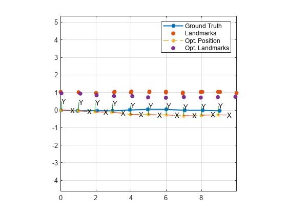
Note that you can improve the accuracy of the optimization by increasing the sliding window size or by using custom factor graph solver options.

Input Arguments

fg — Factor graph

factorGraph object

Factor graph, specified as a factorGraph object.

poseNodeIDs — IDs of pose nodes to optimize

N-element row vector of nonnegative integers

IDs of pose nodes to optimize within the factor graph, specified as an N-element row vector of nonnegative integers. N is the total number of pose nodes to optimize.

The pose nodes specified by poseNodeIDs must all be of type "POSE_SE2", or must all be of type "POSE_SE3". The specified pose nodes must also be unique. For example, poseNodeIDs cannot be [1 2 1] because node ID 1 not unique in this vector.

The specified pose nodes in the factor graph must form a connected factor graph. For more information, see Factor Graph Connectivity.

solverOptions — Solver options for factor graph

factorGraphSolverOptions object

Solver options for the factor graph, specified as a factorGraphSolverOptions object.

Output Arguments

solnInfo — Results of optimization

structure

Results of the optimization, returned as a structure containing:

• InitialCost — Initial cost of the non-linear least squares problem formulated by the factor graph before the optimization.

• FinalCost — Final cost of the non-linear least squares problem formulated by the factor graph after the optimization.

  Note

  Cost is the sum of error terms, known as residuals, where each residual is a function of a subset of factor measurements.

• NumSuccessfulSteps — Number of iterations in which the solver decreases the cost. This value includes the initialization iteration at 0 in addition to the minimizer iterations.

• NumUnsuccessfulSteps — Number of iterations in which the iteration is numerically invalid or the solver does not decrease the cost.

• TotalTime — Total solver optimization time in seconds.

• TerminationType — Termination type as an integer in the range [0, 2]:

  • 0 — Solver found a solution that meets convergence criterion and decreases in cost after optimization.

  • 1 — Solver could not find a solution that meets convergence criterion after running for the maximum number of iterations.

  • 2 — Solver terminated due to an error.

• IsSolutionUsable — The solution is usable if the solution has either converged or optimize has reached the maximum number of iterations. The value is 1 (true) if the solution is usable and the value is 0 (false) if the solution is not usable.

• OptimizedNodeIDs — Node IDs of nodes that were optimized during the optimization.

• FixedNodeIDs — Node IDs of nodes that were fixed during optimization in the factor graph or partial factor graph. Note that these fixed nodes still contribute to the optimization of other specified nodes.

More About

Factor Graph Connectivity

A factor graph is considered connected if there is a path between every pair of nodes. For example, for a factor graph containing four pose nodes, connected consecutively by three factors, there are paths in the factor graph from one node in the graph to any other node in the graph.

connected = isConnected(fg,[1 2 3 4])

connected =

     1

If the graph does not contain node 3, although there is still a path from node 1 to node 2, there is no path from node 1 or node 2 to node 4.

connected = isConnected(fg,[1 2 4])

connected =

     0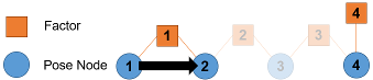

A fully connected factor graph is important for optimization. If the factor graph is not fully connected, then the optimization occurs separately for each of the disconnected graphs, which may produce undesired results. The connectivity of graphs can become more complex when you specify certain subsets of pose node IDs to optimize. This is because the optimize function optimizes parts of the factor graph by using the specified IDs to identify which factors to use to create a partial factor graph. optimize adds a factor to the partial factor graph if that factor connects to any of the specified pose nodes and does not connect to any unspecified pose nodes. 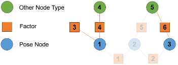The function also adds any non-pose nodes that the added factors connect to, but does not add other factors connected to those nodes. For example, for this factor graph there are three pose nodes, two non-pose nodes, and the factors that connect the nodes.

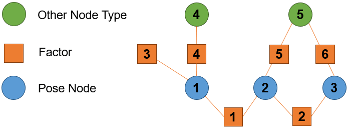
If you specify nodes 1 and 2, then factors 1, 3, 4, and 5 form a factor graph for the optimization because they connect to pose nodes 1 and 2. The optimization includes nodes 4 and 5 because they connect to factors that relate to the specified pose node IDs.

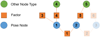
If you specify poseNodeIDs as [1 3], then the optimize function optimizes each separated graph separately because the formed factor graph does not contain a path between nodes 1 and 3.

Tips

• Before you optimize the factor graph or a subset of nodes, use the nodeState function to save the node states to the workspace. If, after running the optimization, you want to make adjustments to it, you can set the node states back to the saved states.

• For debugging a partial optimization of a factor graph, check the OptimizedNodeIDs and FixedNodeIDs fields of the solnInfo output argument to see which of the optimized node IDs and which of fixed nodes contributed to the optimization.

• To check if poseNodeIDs forms a connected factor graph, use the isConnected function.

Extended Capabilities

C/C++ Code Generation
Generate C and C++ code using MATLAB® Coder™.

Version History

Introduced in R2022a

R2023b: Optimize specified nodes

The optimize function now supports specifying node IDs to optimize a subset of nodes from a factor graph. This is useful for applications such as visual SLAM, where you must optimize nodes in a sliding window.