Feasibility Using Problem-Based Optimize Live Editor Task
Problem Description
This example shows how to find a feasible point using the Optimize Live Editor task using a variety of solvers. The problem is to find a point satisfying these constraints:
.
Graph the curves where the constraint functions are equal to zero. To see which part of the region is feasible (negative constraint function value), plot the curves where the constraint functions equal –1/2. Use the plotobjconstr function appearing at the end of this script.
plotobjconstr
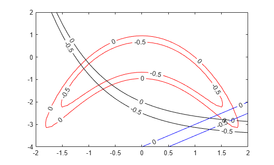
There appears to be a small feasible region near . Notice that there is no point where all constraint values are below –1/2, so the feasible set is small.
Use Problem-Based Optimize Live Editor Task
To find a feasible point, launch the Optimize Live Editor task from a Live Script by choosing Task > Optimize on the Code tab or Insert tab. Choose the problem-based task.
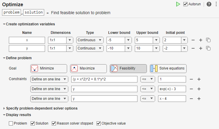
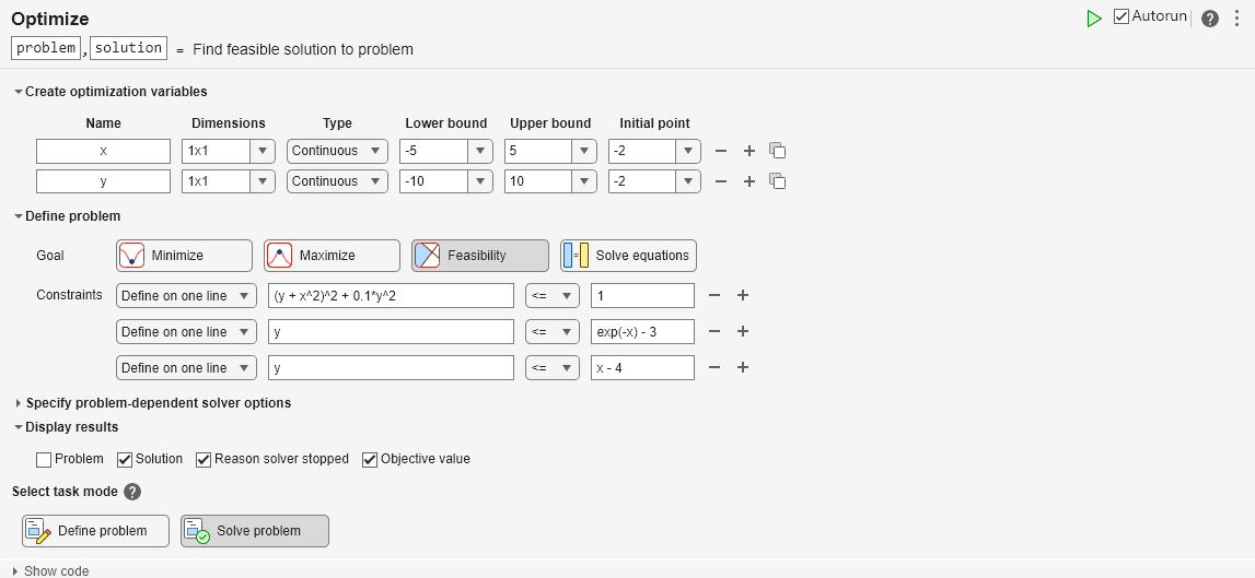
Set the problem variable x to have lower bound –5 and upper bound 5. Set the problem variable y to have lower bound –10 and upper bound 10. Set the initial point for x to 2 and for y to –2.
Set the Goal to Feasibilty.
Create inequalities representing the three constraints. Your task should match this picture.
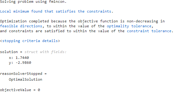
Switch the task mode to Solve problem. The task chooses the fmincon solver, and reaches the following solution.
Effect of Initial Point
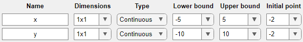
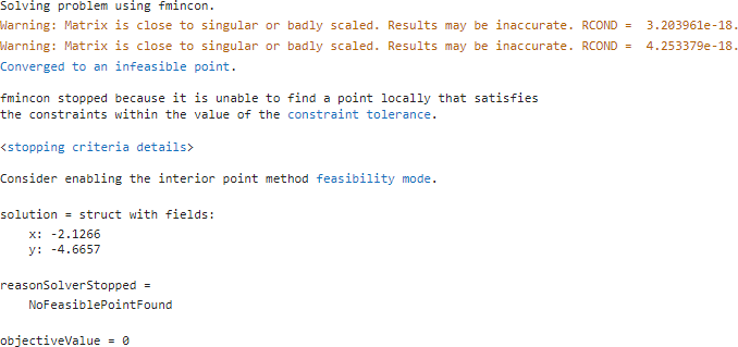
Starting from a different initial point can cause fmincon to fail to find a solution. Set the initial point for x to –2.
This time fmincon fails to find a feasible solution.
Try Different Solver
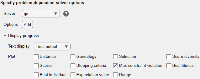
To attempt to find a solution, try a different solver. Set the solver to ga. To do so, specify the solver in the Specify problem-dependent solver options expander. And to monitor the solver progress, set the plot function to Max constraint violation.
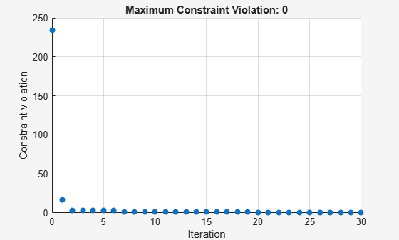
ga finds a feasible point to within the constraint tolerance.
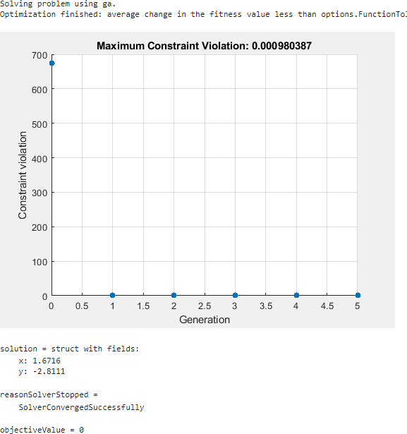
ga finds a different solution than fmincon. The solution is slightly infeasible. To get a solution with lower infeasibility, you can set the constraint tolerance option to a lower value than the default. Alternatively, try a different solver.
Try surrogateopt
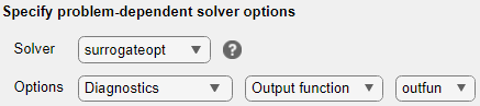
Try using the surrogateopt solver. Set the plot function as Max constraint violation; this setting does not carry forward automatically from the ga solution.
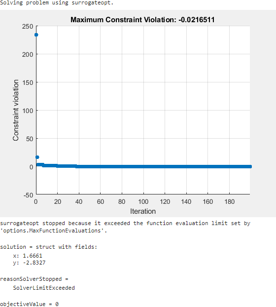
surrogateopt reaches a feasible solution, but does not stop when it first reaches a solution. Instead, surrogateopt continues to iterate until it reaches its function evaluation limit. To stop the iterations earlier, specify an output function that halts the solver as soon as the maximum constraint violation reaches 1e-6 or less. Doing so causes the solver to stop much earlier. Use the surrout helper function, which appears at the end of this script. To specify this function, create a function handle to the function.
outfun = @surrout;
Specify this function handle in the Specify problem-dependent solver options > Options > Diagnostics > Output function drop-down menu.
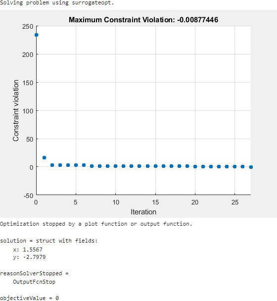
This time the solver stops after about 30 function evaluations instead of 200. The solution is slightly different than the previous one, but both are feasible solutions.
Conclusions
The problem-based Optimize Live Editor task helps you try using different solvers on a problem, even solvers that have different syntaxes such as fmincon and surrogateopt. The task also helps you set plot functions, and set other options.
The task appears here in its final state. Feel free to experiment using different solvers and options.
Solving problem using surrogateopt.
Optimization stopped by a plot function or output function.
solution = struct with fields:
    x: 1.5639
    y: -2.8127
reasonSolverStopped =
    OutputFcnStop
objectiveValue =
0
Helper Functions
This code creates the plotobjconstr helper function.
function plotobjconstr
[XX,YY] = meshgrid(-2:0.1:2,-4:0.1:2);
ZZ = objconstr([XX(:),YY(:)]).Ineq;
ZZ = reshape(ZZ,[size(XX),3]);
h = figure;
ax = gca;
contour(ax,XX,YY,ZZ(:,:,1),[-1/2 0],"r",ShowText="on");
hold on
contour(ax,XX,YY,ZZ(:,:,2),[-1/2 0],"k",ShowText="on");
contour(ax,XX,YY,ZZ(:,:,3),[-1/2 0],"b",ShowText="on");
hold off
end
This code creates the objconstr helper function.
function f = objconstr(x)
c(:,1) = (x(:,2) + x(:,1).^2).^2 + 0.1*x(:,2).^2 - 1;
c(:,2) = x(:,2) - exp(-x(:,1)) + 3;
c(:,3) = x(:,2) - x(:,1) + 4;
f.Ineq = c;
end
This code creates the surrout helper function
function stop = surrout(~,optimValues,~)
stop = false;
if optimValues.constrviolation <= 1e-6 % Tolerance for constraint
    stop = true;
end
end
See Also
Optimize | fmincon | ga (Global Optimization Toolbox) | surrogateopt (Global Optimization Toolbox)