Bound-Constrained Quadratic Programming, Solver-Based
This example shows how to determine the shape of a circus tent by solving a quadratic optimization problem. The tent is formed from heavy, elastic material, and settles into a shape that has minimum potential energy subject to constraints. A discretization of the problem leads to a bound-constrained quadratic programming problem.
For a problem-based version of this example, see Bound-Constrained Quadratic Programming, Problem-Based.
Problem Definition
Consider building a circus tent to cover a square lot. The tent has five poles covered with a heavy, elastic material. The problem is to find the natural shape of the tent. Model the shape as the height x(p) of the tent at position p.
The potential energy of heavy material lifted to height x is cx, for a constant c that is proportional to the weight of the material. For this problem, choose c = 1/3000.
The elastic potential energy of a piece of the material is approximately proportional to the second derivative of the material height, times the height. You can approximate the second derivative by the 5-point finite difference approximation (assume that the finite difference steps are of size 1). Let represent a shift of 1 in the first coordinate direction, and represent a shift by 1 in the second coordinate direction.
The natural shape of the tent minimizes the total potential energy. By discretizing the problem, you find that the total potential energy to minimize is the sum over all positions p of + cx(p).
This potential energy is a quadratic expression in the variable x.
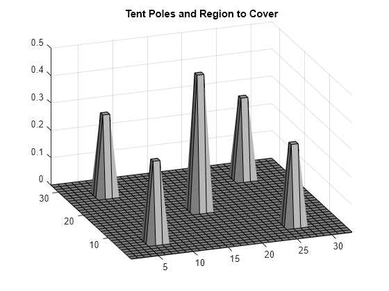
Specify the boundary condition that the height of the tent at the edges is zero. The tent poles have a cross section of 1-by-1 unit, and the tent has a total size of 33-by-33 units. Specify the height and location of each pole. Plot the square lot region and tent poles.
height = zeros(33);
height(6:7,6:7) = 0.3;
height(26:27,26:27) = 0.3;
height(6:7,26:27) = 0.3;
height(26:27,6:7) = 0.3;
height(16:17,16:17) = 0.5;
colormap(gray);
surfl(height)
axis tight
view([-20,30]);
title("Tent Poles and Region to Cover")

Create Boundary Conditions
The height matrix defines the lower bounds on the solution x. To restrict the solution to be zero at the boundary, set the upper bound ub to be zero on the boundary.
boundary = false(size(height));
boundary([1,33],:) = true;
boundary(:,[1,33]) = true;
ub = inf(size(boundary)); % No upper bound on most of the region
ub(boundary) = 0;
Create Objective Function Matrices
The quadprog problem formulation is to minimize
.
In this case, the linear term corresponds to the potential energy of the material height. Therefore, specify f = 1/3000 for each component of x.
f = ones(size(height))/3000;
Create the finite difference matrix representing by using the delsq function. The delsq function returns a sparse matrix with entries of 4 and -1 corresponding to the entries of 4 and -1 in the formula for . Multiply the returned matrix by 2 to have quadprog solve the quadratic program with the energy function as given by .
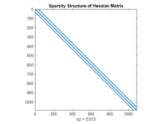
H = delsq(numgrid("S",33+2))*2;View the structure of the matrix H. The matrix operates on x(:), which means the matrix x is converted to a vector by linear indexing.
spy(H);
title("Sparsity Structure of Hessian Matrix");
Run Optimization Solver
Solve the problem by calling quadprog.
x = quadprog(H,f,[],[],[],[],height,ub);
Minimum found that satisfies the constraints.

Optimization completed because the objective function is non-decreasing in
feasible directions, to within the value of the optimality tolerance,
and constraints are satisfied to within the value of the constraint tolerance.

<stopping criteria details>
Plot Solution
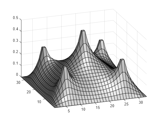
Reshape the solution x to a matrix S. Then plot the solution.
S = reshape(x,size(height));
surfl(S);
axis tight;
view([-20,30]);