Minimization with Bound Constraints and Banded Preconditioner

This example shows how to solve a nonlinear problem with bounds using the fmincon trust-region-reflective algorithm. This algorithm provides additional efficiency when the problem is sparse, and has both an analytic gradient and a known structure, such as its Hessian pattern.

Objective Function with Gradient

For a given $$n$$ that is a positive multiple of 4, the objective function is

$$f(x)=1+\sum _{i=1}^n{\left|\left(3-2x_i\right)x_i-x_{i-1}-x_{i+1}+1\right|}^p+\sum _{i=1}^{n/2}{\left|x_i+x_{i+n/2}\right|}^p,$$

where $$p=7/3$$, $$x_0=0$$, and $$x_{n+1}=0$$. The tbroyfg helper function at the end of this example implements the objective function, including its gradient.

The problem has the bounds $$-10\le x_i\le 10$$ for all $$i$$. Use $$n$$ = 800.

n = 800;
lb = -10*ones(n,1);
ub = -lb;

Hessian Pattern

The sparsity pattern of the Hessian matrix is predetermined and stored in the file tbroyhstr.mat. The sparsity structure for the Hessian of this problem is banded, as you can see in the following spy plot.

load tbroyhstr
spy(Hstr)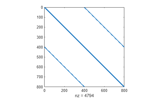

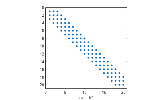
In this plot, the center stripe is itself a five-banded matrix. The following plot shows the matrix more clearly.

spy(Hstr(1:20,1:20))

Problem Options

Set options to use the trust-region-reflective algorithm. This algorithm requires you to set the SpecifyObjectiveGradient option to true.

Also, use optimoptions to set the HessPattern option to Hstr. If you do not set this option for such a large problem with an obvious sparsity structure, the problem uses a great amount of memory and computation because fmincon attempts to use finite differencing on a full Hessian matrix of 640,000 nonzero entries.

options = optimoptions('fmincon','SpecifyObjectiveGradient',true,'HessPattern',Hstr,...
    'Algorithm','trust-region-reflective');

Solve Problem

Set the initial point to –1 for odd indices and +1 for even indices.

x0 = -ones(n,1);
x0(2:2:n) = 1;

The problem has no linear or nonlinear constraints, so set those parameters to [].

A = [];
b = [];
Aeq = [];
beq = [];
nonlcon = [];

Call fmincon to solve the problem.

[x,fval,exitflag,output] = ... 
   fmincon(@tbroyfg,x0,A,b,Aeq,beq,lb,ub,nonlcon,options);

Local minimum possible.

fmincon stopped because the final change in function value relative to 
its initial value is less than the value of the function tolerance.

Examine Solution and Solution Process

Examine the exit flag, objective function value, first-order optimality measure, and number of solver iterations.

disp(exitflag);

     3

disp(fval)

  270.4790

disp(output.firstorderopt)

    0.0163

disp(output.iterations)

     7

fmincon does not take many iterations to reach a solution. However, the solution has a relatively high first-order optimality measure, which is why the exit flag does not have the preferred value of 1.

Improve Solution

Try using a five-banded preconditioner instead of the default diagonal preconditioner. Using optimoptions, set the PrecondBandWidth option to 2 and solve the problem again. (The bandwidth is the number of upper or lower diagonals, not counting the main diagonal.)

options.PrecondBandWidth = 2;
[x2,fval2,exitflag2,output2] = ... 
   fmincon(@tbroyfg,x0,A,b,Aeq,beq,lb,ub,nonlcon,options);

Local minimum possible.

fmincon stopped because the final change in function value relative to 
its initial value is less than the value of the function tolerance.

disp(exitflag2);

     3

disp(fval2)

  270.4790

disp(output2.firstorderopt)

   7.5340e-05

disp(output2.iterations)

     9

The exit flag and objective function value do not appear to change. However, the number of iterations increases, and the first-order optimality measure decreases considerably. Compute the difference in objective function value.

disp(fval2 - fval)

  -2.9005e-07

The objective function value decreases by a tiny amount. The solution mainly improves the first-order optimality measure, not the objective function.

Helper Function

This code creates the tbroyfg helper function.

function [f,grad] = tbroyfg(x,dummy)
%TBROYFG Objective function and its gradients for nonlinear minimization
% with bound constraints and banded preconditioner.
% Documentation example.

%   Copyright 1990-2008 The MathWorks, Inc.

n = length(x);  % n should be a multiple of 4
p = 7/3;
y=zeros(n,1);
i = 2:(n-1);
y(i) = abs((3-2*x(i)).*x(i) - x(i-1) - x(i+1)+1).^p;
y(n) = abs((3-2*x(n)).*x(n) - x(n-1)+1).^p;
y(1) = abs((3-2*x(1)).*x(1) - x(2)+1).^p;
j = 1:(n/2);
z = zeros(length(j),1);
z(j) = abs(x(j) + x(j+n/2)).^p;
f = 1 + sum(y) + sum(z);
%
% Evaluate the gradient.
if nargout > 1
   g = zeros(n,1);
   t = zeros(n,1);
   i = 2:(n-1);
   t(i) = (3-2*x(i)).*x(i) - x(i-1) - x(i+1) + 1;
   g(i) = p*abs(t(i)).^(p-1).*sign(t(i)).*(3-4*x(i));
   g(i-1) = g(i-1) - p*abs(t(i)).^(p-1).*sign(t(i));
   g(i+1) = g(i+1) - p*abs(t(i)).^(p-1).*sign(t(i));
   tt = (3-2*x(n)).*x(n) - x(n-1) + 1;
   g(n) = g(n) + p*abs(tt).^(p-1).*sign(tt).*(3-4*x(n));
   g(n-1) = g(n-1) - p*abs(tt).^(p-1).*sign(tt);
   tt = (3-2*x(1)).*x(1)-x(2)+1;
   g(1) = g(1) + p*abs(tt).^(p-1).*sign(tt).*(3-4*x(1));
   g(2) = g(2) - p*abs(tt).^(p-1).*sign(tt);
   j = 1:(n/2);
   t(j) = x(j) + x(j+n/2);
   g(j) = g(j) + p*abs(t(j)).^(p-1).*sign(t(j));
   jj = j + (n/2);
   g(jj) = g(jj) + p*abs(t(j)).^(p-1).*sign(t(j));
   grad = g;
end
end

×

Open Example

You have a modified version of this example. Do you want to open this example with your edits?

No, overwrite the modified version Yes