batteryP2DResults
R2026bDescription
A batteryP2DResults object contains the
concentration of Li-ion and electric potential in solid active material particles in both the
anode and cathode, as well as in the liquid electrolyte. The object also contains the voltage
at the battery terminals, ionic flux, solution times, and mesh.
Creation
Solve a battery pseudo-2D (P2D) problem using the solve function. The solution returned by this function is a
batteryP2DResults object.
Properties
Object Functions
plotSummary | Plot battery P2D modeling solution |
Examples
Solve a Li-Ion battery electrochemistry problem by using a pseudo-2D battery model.
Both the anode and cathode materials require the open circuit potential specification, which determines the voltage profile of the battery during charging and discharging. The open circuit potential is a voltage of electrode material as a function of the stoichiometric ratio, which is the ratio of intercalated lithium in the solid to maximum lithium capacity. You can specify this ratio by interpolating the gridded data set.
sNorm = linspace(0.025, 0.975, 39);
ocp_n_vec = [.435;.325;.259;.221;.204; ...
    .194;.179;.166;.155;.145; ...
    .137;.131;.128;.127;.126; ...
    .125;.124;.123;.122;.121; ...
    .118;.117;.112;.109;.105; ...
    .1;.098;.095;.094;.093; ...
    .091;.09;.089;.088;.087; ...
    .086;.085;.084;.083];
ocp_p_vec = [3.598;3.53;3.494;3.474; ...
    3.46;3.455;3.454;3.453; ...
    3.4528;3.4526;3.4524;3.452; ...
    3.4518;3.4516;3.4514;3.4512; ...
    3.451;3.4508;3.4506;3.4503; ...
    3.45;3.4498;3.4495;3.4493; ...
    3.449;3.4488;3.4486;3.4484; ...
    3.4482;3.4479;3.4477;3.4475; ...
    3.4473;3.447;3.4468;3.4466; ...
    3.4464;3.4462;3.4458];

anodeOCP = griddedInterpolant(sNorm,ocp_n_vec,"linear","nearest");
cathodeOCP = griddedInterpolant(sNorm,ocp_p_vec,"linear","nearest");
Create objects that specify the active materials for the anode and cathode.
anodeMaterial = batteryActiveMaterial( ...
    ParticleRadius=5E-6, ...
    MaximumSolidConcentration=30555, ...
    VolumeFraction=0.58, ...
    DiffusionCoefficient=3.0E-15, ...
    ReactionRate=8.8E-11, ...
    OpenCircuitPotential=@(st_ratio) anodeOCP(st_ratio), ...
    StoichiometricLimits=[0.0132 0.811]);

cathodeMaterial = batteryActiveMaterial(...
    ParticleRadius=5E-8, ...
    MaximumSolidConcentration=22806, ...
    VolumeFraction=0.374, ...
    DiffusionCoefficient=5.9E-19, ...
    ReactionRate=2.2E-13, ...
    OpenCircuitPotential=@(st_ratio) cathodeOCP(st_ratio), ...
    StoichiometricLimits=[0.035 0.74]);
Next, create objects that specify both electrodes.
anode = batteryElectrode(...
    Thickness=34E-6, ...
    Porosity=0.3874, ...
    BruggemanCoefficient=1.5, ...
    ElectricalConductivity=100, ...
    ActiveMaterial=anodeMaterial);

cathode = batteryElectrode(...
    Thickness=80E-6, ...
    Porosity=0.5725, ...
    BruggemanCoefficient=1.5, ...
    ElectricalConductivity=0.5, ...
    ActiveMaterial=cathodeMaterial);
Create an object that specifies the properties of the separator.
separator = batterySeparator(...
    Thickness=25E-6, ...
    Porosity=0.45, ...
    BruggemanCoefficient=1.5);
Create an object that specifies the properties of the electrolyte.
electrolyte = batteryElectrolyte(...
    DiffusionCoefficient=2E-10, ...
    TransferenceNumber=0.363, ...
    IonicConductivity=0.29);
Create an object that specifies the initial conditions of the battery.
ic = batteryInitialConditions(...
    ElectrolyteConcentration=1000, ...
    StateOfCharge=0.05, ...
    Temperature=298.15);
Create an object that specifies the properties of the battery cycling step.
cycling = batteryCyclingStep(...
    NormalizedCurrent=0.5, ...
    CutoffTime=100, ...
    CutoffVoltageUpper=4.2, ...
    OutputTimeStep=10);
Create a model for the battery P2D analysis.
model = batteryP2DModel(...
    Anode=anode, ...
    Separator=separator, ...
    Cathode=cathode, ...
    Electrolyte=electrolyte, ...
    InitialConditions=ic, ...
    CyclingStep=cycling);
Set the maximum step size for the internal solver to 2.
model.SolverOptions.MaxStep = 2;
Solve the model using the solve function. The resulting object contains the concentration of Li-ion and electric potential in solid active material particles in both the anode and cathode, as well as in the liquid electrolyte. The object also contains the voltage at the battery terminals, ionic flux, solution times, and mesh.
results = solve(model)
results =
  batteryP2DResults with properties:

   Base P2D Properties
                SolutionTimes: [11×1 double]
              TerminalVoltage: [11×1 double]
            NormalizedCurrent: [11×1 double]
          LiquidConcentration: [11×49 double]
               SolidPotential: [11×49 double]
              LiquidPotential: [11×49 double]
                    IonicFlux: [11×49 double]
    AverageSolidConcentration: [11×49 double]
    SurfaceSolidConcentration: [11×49 double]
           SolidConcentration: [11×7×49 double]
                         Mesh: [1×1 batteryMesh]
Visualize the results.
plotSummary(results)
![Figure contains 6 axes objects. Axes object 1 with title Terminal Voltage [V], xlabel Time [s] contains an object of type line. Axes object 2 with title Normalized Current, xlabel Time [s] contains an object of type line. Axes object 3 with title Liquid Concentration [mol/m Cubed baseline ], xlabel Thickness [m] contains 7 objects of type line, rectangle. Axes object 4 with title Normalized Average Solid Concentration, xlabel Thickness [m] contains 7 objects of type line, rectangle. Axes object 5 with title Liquid Potential [V], xlabel Thickness [m] contains 7 objects of type line, rectangle. Axes object 6 with title Solid Potential [V], xlabel Thickness [m] contains 7 objects of type line, rectangle. These objects represent 0, 30, 60, 100.](../../examples/pde/SolveModelForBatteryP2DAnalysisExample_01.png)
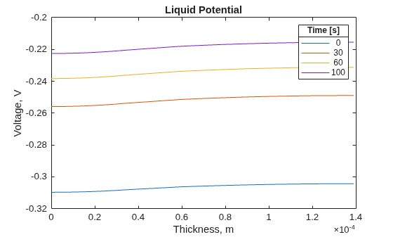
To see more details of the liquid potential distribution, plot it separately. Use the same four solution times.
figure
for i = [1 4 7 11]
plot(results.Mesh.Nodes, ...
results.LiquidPotential(i,:))
    hold on
end
title("Liquid Potential")
xlabel("Thickness, m")
ylabel("Voltage, V")
lgd = legend(num2str(results.SolutionTimes([1;4;7;11])));
lgd.Title.String = "Time [s]";
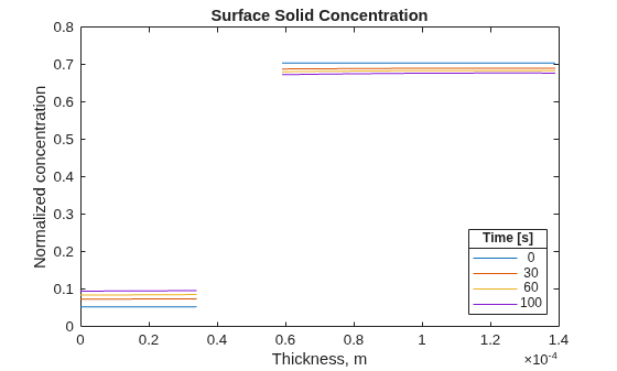
Plot the surface solid concentration distribution for the same four solution times.
figure
for i = [1 4 7 11]
plot(results.Mesh.Nodes, ...
results.SurfaceSolidConcentration(i,:))
    hold on
end
title("Surface Solid Concentration")
xlabel("Thickness, m")
ylabel("Normalized concentration")
lgd = legend(num2str(results.SolutionTimes([1;4;7;11])));
lgd.Location = "southeast";
lgd.Title.String = "Time [s]";
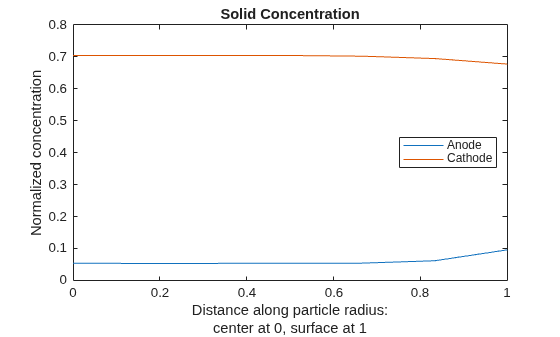
For the final solution time, 100s, plot the solid concentration along the particle radius at two locations corresponding approximately to the middle of the anode and the middle of the cathode.
figure
Rfinal = results.SolidConcentration(end,:,:);
Nr = size(results.SolidConcentration,2);
for x = [results.Mesh.AnodeNodes(ceil(end/2)) ...
         results.Mesh.CathodeNodes(ceil(end/2))]
    Rr = Rfinal(:,:,x);
plot((0:Nr-1).'/(Nr-1),Rr(:))
    hold on
end
title("Solid Concentration")
xlabel({"Distance along particle radius:";"center at 0, surface at 1"})
ylabel("Normalized concentration")
legend("Anode","Cathode",Location="east");
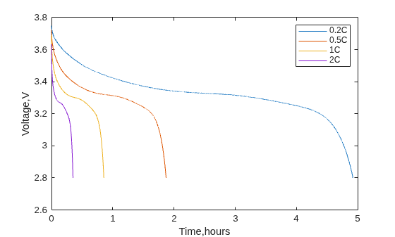
Model the battery discharging for four different constant values of the normalized current.
Specify the universal gas constant, the Faraday constant, the Boltzmann constant, the elementary charge, and the simulation temperature.
R = 8.31446; % J/(mol·K))
FaradayConstant = 96487; % C/mol
BoltzmannConstant = 1.380649E-23; % J/K
ElementaryCharge = 1.6021766E-19; % C
SimulationTemperature = 298.15; % K
The open circuit potential is a voltage of electrode material as a function of the stoichiometric ratio, which is the ratio of intercalated lithium in the solid to maximum lithium capacity. Create this function to specify the open circuit potential of the anode.
function anodeOCP = anodefuncOCP(st_ratio)
anodeOCP = -591.7*st_ratio.^9+2984*st_ratio.^8 ...
           -6401*st_ratio.^7+7605*st_ratio.^6- ...
            5465*st_ratio.^5+2438*st_ratio.^4 ...
           -670.5*st_ratio.^3+110.2*st_ratio.^2- ...
            10.39*st_ratio+0.6363;
end
Specify the properties of the battery anode by creating a batteryActiveMaterial object. The properties of this object specify the active material of the anode, including the particle radius, maximum solid-phase concentration of lithium ions, fraction of the anode volume occupied by the active material, diffusion coefficient, reaction rate, open circuit potential of the anode material as a function of the stoichiometric ratio, and the range of stoichiometric values.
anodeMaterial = batteryActiveMaterial( ...
    ParticleRadius=5E-6, ...
    VolumeFraction=0.58, ...
    MaximumSolidConcentration=30555, ...
    DiffusionCoefficient=3.0E-15, ...
    ReactionRate=8.8E-11, ...
    OpenCircuitPotential=@anodefuncOCP, ...
    StoichiometricLimits=[0.0132 0.811]);
Specify the open circuit potential of the cathode by interpolating the gridded data set.
sNorm = linspace(0.025, 0.975, 39);
ocp_p_vec = [3.598;3.53;3.494;3.474; ...
    3.46;3.455;3.454;3.453; ...
    3.4528;3.4526;3.4524;3.452; ...
    3.4518;3.4516;3.4514;3.4512; ...
    3.451;3.4508;3.4506;3.4503; ...
    3.45;3.4498;3.4495;3.4493; ...
    3.449;3.4488;3.4486;3.4484; ...
    3.4482;3.4479;3.4477;3.4475; ...
    3.4473;3.447;3.4468;3.4466; ...
    3.4464;3.4462;3.4458];

cathodeOCP = griddedInterpolant(sNorm,ocp_p_vec,"linear","nearest");
Specify the diffusion coefficient as a function of the solid concentration.
DiffusivityReference = @(s)5.9E-19*((s-0.5).^2+0.75);
Create a batteryActiveMaterial object that specifies the active material of the cathode, including the particle radius, maximum solid-phase concentration of lithium ions, fraction of the anode volume occupied by the active material, diffusion coefficient, reaction rate, voltage of the anode material as a function of the stoichiometric ratio, and the range of stoichiometric values.
cathodeMaterial = batteryActiveMaterial( ...
    ParticleRadius=5E-8, ...
    VolumeFraction=0.374, ...
    MaximumSolidConcentration=22806, ...
    DiffusionCoefficient= @(r,s) DiffusivityReference(s.SolidConcentration/22806), ...
    ReactionRate=2.2E-13, ...
    OpenCircuitPotential=@(st_ratio) cathodeOCP(st_ratio), ...
    StoichiometricLimits=[0.035 0.74]);
Create the objects that specify the anode and cathode properties, such as the thickness, porosity, Bruggeman's coefficient, electrical conductivity, and active material.
anode = batteryElectrode( ...
    Thickness=34E-6, ...
    Porosity=0.3874, ...
    BruggemanCoefficient=1.5, ...
    ElectricalConductivity=100, ...
    ActiveMaterial=anodeMaterial);

cathode=batteryElectrode( ...
    Thickness=80E-6, ...
    Porosity=0.5725, ...
    BruggemanCoefficient=1.5, ...
    ElectricalConductivity=0.5, ...
    ActiveMaterial=cathodeMaterial);
Specify the thickness, porosity, and Bruggeman's coefficient of the battery separator.
separator=batterySeparator( ...
    Thickness=25E-6, ...
    Porosity=0.45, ...
    BruggemanCoefficient=1.5);
Specify the diffusion coefficient, transference number, and ionic conductivity of the battery electrolyte.
ConductivityElectrolyte = ...
    @(ce) -4.582e-01*(ce/1000).^2 + 1.056*(ce/ 1000) + 0.3281;

electrolyte = batteryElectrolyte( ...
    DiffusionCoefficient= ...
        @(r,s) BoltzmannConstant/(FaradayConstant*ElementaryCharge)* ...
        SimulationTemperature* ...
        ConductivityElectrolyte(s.LiquidConcentration)./s.LiquidConcentration, ...
    TransferenceNumber=0.363, ...
    IonicConductivity=@(x,s) ConductivityElectrolyte(s.LiquidConcentration));
Specify the minimum voltage limit for the battery during discharging. Also specify the output time step for the solver.
cycling = batteryCyclingStep( ...
    CutoffVoltageLower=2.8, ...
    OutputTimeStep=1);
Specify the initial temperature for the battery.
ic = batteryInitialConditions( ...
    Temperature=SimulationTemperature);
Create a model for the battery P2D analysis and set its properties using the objects created.
model = batteryP2DModel( ...
    Anode=anode, ...
    Cathode=cathode, ...
    Separator=separator, ...
    Electrolyte=electrolyte, ...
    CyclingStep=cycling, ...
    InitialConditions=ic);
Specify the state of charge (SoC) as 1 to indicate that the battery is fully charged.
model.InitialConditions.StateOfCharge = 1;
Specify the electrolyte concentration for the fully charged battery.
model.InitialConditions.ElectrolyteConcentration = 1200;
Set the maximum step size for the internal solver to 2.
model.SolverOptions.MaxStep = 2;
Solve the model for four values of the normalized current: –0.2, –0.5, –1, and –2. Negative values indicate that the battery is discharging.
model.CyclingStep.NormalizedCurrent = -0.2;
R02 = solve(model);
model.CyclingStep.NormalizedCurrent = -0.5;
R05 = solve(model);
model.CyclingStep.NormalizedCurrent = -1;
R1 = solve(model);
model.CyclingStep.NormalizedCurrent = -2;
R2 = solve(model);
Plot the resulting terminal voltage at each solution time.
plot(R02.SolutionTimes./3600,R02.TerminalVoltage)
hold on
plot(R05.SolutionTimes./3600,R05.TerminalVoltage)
plot(R1.SolutionTimes./3600,R1.TerminalVoltage)
plot(R2.SolutionTimes./3600,R2.TerminalVoltage)
xlabel("Time,hours")
ylabel("Voltage,V")
legend("0.2C","0.5C","1C","2C");
hold off
Since R2026b
Account for battery aging due to the growth of the solid electrolyte interphase (SEI) layer. Including the SEI growth model lets you simulate capacity fading and power loss over repeated battery cycles.
Both the anode and cathode materials require the open circuit potential specification, which determines the voltage profile of the battery during charging and discharging. The open circuit potential is a voltage of electrode material as a function of the stoichiometric ratio, which is the ratio of intercalated lithium in the solid to maximum lithium capacity. You can specify this ratio by interpolating the gridded data set.
sNorm = linspace(0.025, 0.975, 39);
ocp_n_vec = [.435;.325;.259;.221;.204; ...
    .194;.179;.166;.155;.145; ...
    .137;.131;.128;.127;.126; ...
    .125;.124;.123;.122;.121; ...
    .118;.117;.112;.109;.105; ...
    .1;.098;.095;.094;.093; ...
    .091;.09;.089;.088;.087; ...
    .086;.085;.084;.083];
ocp_p_vec = [3.598;3.53;3.494;3.474; ...
    3.46;3.455;3.454;3.453; ...
    3.4528;3.4526;3.4524;3.452; ...
    3.4518;3.4516;3.4514;3.4512; ...
    3.451;3.4508;3.4506;3.4503; ...
    3.45;3.4498;3.4495;3.4493; ...
    3.449;3.4488;3.4486;3.4484; ...
    3.4482;3.4479;3.4477;3.4475; ...
    3.4473;3.447;3.4468;3.4466; ...
    3.4464;3.4462;3.4458];

anodeOCP = griddedInterpolant(sNorm,ocp_n_vec,"linear","nearest");
cathodeOCP = griddedInterpolant(sNorm,ocp_p_vec,"linear","nearest");
Create objects that specify the active materials for the anode and cathode.
anodeMaterial = batteryActiveMaterial( ...
    ParticleRadius=5E-6, ...
    MaximumSolidConcentration=30555, ...
    VolumeFraction=0.58, ...
    DiffusionCoefficient=3.0E-15, ...
    ReactionRate=8.8E-11, ...
    OpenCircuitPotential=@(st_ratio) anodeOCP(st_ratio), ...
    StoichiometricLimits=[0.0132 0.811]);

cathodeMaterial = batteryActiveMaterial(...
    ParticleRadius=5E-8, ...
    MaximumSolidConcentration=22806, ...
    VolumeFraction=0.374, ...
    DiffusionCoefficient=5.9E-19, ...
    ReactionRate=2.2E-13, ...
    OpenCircuitPotential=@(st_ratio) cathodeOCP(st_ratio), ...
    StoichiometricLimits=[0.035 0.74]);
Define the SEI model for the anode.
aging = batterySEIModel( ...
    IonicResistivity=2e5, ...
    MolecularWeight=0.162, ...
    Density=2110, ...
    KineticRateConstant=1.0e-16, ...
    SolventConcentration=4541, ...
    CathodicTransferCoeff=0.5, ...
    StoichiometricCoefficient=2, ...
    SolventDiffusivity=1E-21, ...
    EquilibriumPotential=0.4 ...
    );
Next, create objects that specify both electrodes.
anode = batteryElectrode( ...
    Thickness=34E-6, ...
    Porosity=0.3874, ...
    BruggemanCoefficient=1.5, ...
    ElectricalConductivity=100, ...
    ActiveMaterial=anodeMaterial, ...
    Aging=aging);

cathode = batteryElectrode(...
    Thickness=80E-6, ...
    Porosity=0.5725, ...
    BruggemanCoefficient=1.5, ...
    ElectricalConductivity=0.5, ...
    ActiveMaterial=cathodeMaterial);
Create an object that specifies the properties of the separator.
separator = batterySeparator(...
    Thickness=25E-6, ...
    Porosity=0.45, ...
    BruggemanCoefficient=1.5);
Create an object that specifies the properties of the electrolyte.
electrolyte = batteryElectrolyte( ...
    DiffusionCoefficient=2E-10, ...
    TransferenceNumber=0.363, ...
    IonicConductivity=0.29);
Create an object that specifies the initial conditions of the battery.
ic = batteryInitialConditions( ...
    ElectrolyteConcentration=1000, ...
    StateOfCharge=0.05, ...
    Temperature=298.15, ...
    InitialSEIThickness=5e-9);
Create objects that specify the properties of the battery during charging and discharging.
cycling1 = batteryCyclingStep( ...
    NormalizedCurrent=0.5, ...
    CutoffVoltageUpper=4.2, ...
    CutoffTime=100, ...
    OutputTimeStep=10);
cycling2 = batteryCyclingStep( ...
    NormalizedCurrent=-0.05, ...-
    CutoffVoltageLower=3.2, ...
    OutputTimeStep=10);
Create a model for the battery P2D analysis.
model = batteryP2DModel( ...
    Anode=anode, ...
    Separator=separator, ...
    Cathode=cathode, ...
    Electrolyte=electrolyte, ...
    InitialConditions=ic, ...
    CyclingStep=[cycling1,cycling2]);
Solve the model.
R = solve(model)
Performing cycling step: 1 of 2
Performing cycling step: 2 of 2
R =
  batteryP2DResults with properties:

   Base P2D Properties
                SolutionTimes: [13×1 double]
              TerminalVoltage: [13×1 double]
            NormalizedCurrent: [13×1 double]
          LiquidConcentration: [13×49 double]
               SolidPotential: [13×49 double]
              LiquidPotential: [13×49 double]
                    IonicFlux: [13×49 double]
    AverageSolidConcentration: [13×49 double]
    SurfaceSolidConcentration: [13×49 double]
           SolidConcentration: [13×7×49 double]
                         Mesh: [1×1 batteryMesh]
       IntercalationIonicFlux: [13×49 double]

   SEI Model Properties
                 SEIIonicFlux: [13×49 double]
                 SEIThickness: [13×49 double]
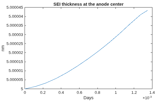
Plot the thickness of the SEI layer at the anode center over time.
plot(R.SolutionTimes/60/60/24, R.SEIThickness(:,10)/1E-9)
xlabel("Days")
title("SEI thickness at the anode center")
ylabel("nm")
Version History
Introduced in R2026aSee Also
Objects
batteryP2DModel|batteryElectrode|batteryElectrolyte|batterySeparator|batteryActiveMaterial|batterySEIModel|batteryCyclingStep|batteryInitialConditions|batteryMesh|batterySolverOptions

