Heat Transfer in Block with Cavity: PDE Modeler App

This example shows how to solve a heat equation that describes the diffusion of heat in a body. This example uses the PDE Modeler app. For programmatic workflow, see Heat Transfer in Block with Cavity.

Consider a block containing a rectangular crack or cavity. The left side of the block is heated to 100 degrees centigrade. At the right side of the block, heat flows from the block to the surrounding air at a constant rate, for example -10 W/m². All the other boundaries are insulated. The temperature in the block at the starting time t₀ = 0 is 0 degrees. The goal is to model the heat distribution during the first five seconds.

The PDE governing this problem is a parabolic heat equation. Partial Differential Equation Toolbox™ solves the generic parabolic PDE of the form

$d \frac{\partial u}{\partial t} - \nabla \cdot (c \nabla u) + a u = f$

The heat equation has the form:

$d \frac{\partial u}{\partial t} - Δ u = 0$

To solve this problem in the PDE Modeler app, follow these steps:

Open the PDE Modeler app by using the pdeModeler command.
```
pdeModeler
```
Model the geometry: draw a rectangle with corners (-0.5,-0.8), (0.5,-0.8), (0.5,0.8), and (-0.5,0.8) and a rectangle with corners (-0.05,-0.4), (0.05,-0.4), (0.05,0.4), and (-0.05,0.4). Draw the first rectangle by using the pderect function.
```
pderect([-0.5 0.5 -0.8 0.8])
```
Display grid lines with extra ticks at -0.05 and 0.05. To do this, select Options > Grid Spacing, clear the Auto checkbox, and enter X-axis extra ticks at -0.05 and 0.05. Then select Options > Grid.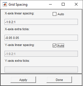
Set the x-axis limit to [-0.6 0.6] and y-axis limit to [-1 1]. To do this, select Options > Axes Limits and set the corresponding ranges.
Select Options > Snap to align any new shape to the grid lines. Then draw the rectangle with corners (-0.05,-0.4), (0.05,-0.4), (0.05,0.4), and (-0.05,0.4)
Model the geometry by entering R1-R2 in the Set formula field.
Check that the application mode is set to Generic Scalar.
Specify the boundary conditions. To do this, switch to the boundary mode by selecting Boundary > Boundary Mode. Then select Boundary > Specify Boundary Conditions and specify the Neumann boundary condition.
- For convenience, first specify the insulating Neumann boundary condition ∂u/∂n = 0 for all boundaries. To do this, select all boundaries by using Edit > Select All and specify g = 0, q = 0.
- Specify the Dirichlet boundary condition u = 100 for the left side of the block. To do this, specify h = 1, r = 100.
- Specify the Neumann boundary condition ∂u/∂n = –10 for the right side of the block. To do this, specify g = -10, q = 0.
Specify the coefficients by selecting PDE > PDE Specification or clicking the button on the toolbar. Heat equation is a parabolic equation, so select the Parabolic type of PDE. Specify c = 1, a = 0, f = 0, and d = 1.
Initialize the mesh by selecting Mesh > Initialize Mesh. Refine the mesh by selecting Mesh > Refine Mesh.
Set the initial value to 0, the solution time to 5 seconds, and compute the solution every 0.5 seconds. To do this, select Solve > Parameters. In the Solve Parameters dialog box, set time to 0:0.5:5, and u(t₀) to 0.
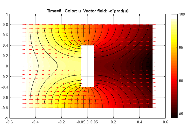
Solve the PDE by selecting Solve > Solve PDE or clicking the button on the toolbar. The app solves the heat equation at 11 different times from 0 to 5 seconds and displays the heat distribution at the end of the time span.
Plot isothermal lines using a contour plot and the heat flux vector field using arrows and change the colormap to hot. To do this:
1. Select Plot > Parameters.
2. In the resulting dialog box, select the Color, Contour, and Arrows options. Select -c*grad(u) from Arrows drop-down menu.
3. Change the colormap to hot by using the corresponding drop-down menu in the same dialog box.
Use an animated plot to visualize the dynamic behavior of the temperature. For this, select Plot > Parameters and then select the Animation option.
The temperature in the block rises very quickly. To improve the animation and focus on the first second, change the list of times to the MATLAB^® expression logspace(-2,0.5,20). To do this, select Solve > Parameters. In the Solve Parameters dialog box, set time to logspace(-2,0.5,20).
You can explore the solution by varying the parameters of the model and plotting the results. For example, change the heat capacity coefficient d and the heat flow at the right boundary to see how these parameters affect the heat distribution.