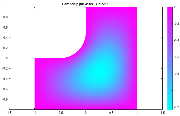
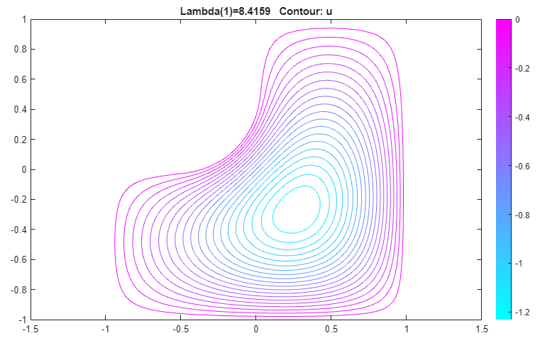
L-Shaped Membrane with Rounded Corner: PDE Modeler App

This example shows how to compute all eigenvalues smaller than 100 and their corresponding eigenvectors. Consider the eigenvalue problem

–Δu = λu

on an L-shaped membrane with a rounded inner corner. The boundary condition is the Dirichlet condition u = 0.

To solve this problem in the PDE Modeler app, follow these steps:

1. Draw an L-shaped membrane as a polygon with the corners (0,0), (–1,0), (–1,–1), (1,–1), (1,1), and (0,1) by using the pdepoly function.

   pdepoly([0 -1 -1 1 1 0],[0 0 -1 -1 1 1])

2. Draw a circle and a square as follows.

   pdecirc(-0.5,0.5,0.5,'C1') 
   pderect([-0.5 0 0.5 0],'SQ1')

3. Model the geometry with the rounded corner by entering P1+SQ1-C1 in the Set formula field.

4. Check that the application mode is set to Generic Scalar.

5. Remove unnecessary subdomain borders by selecting Boundary > Remove All Subdomain Borders.

6. Use the default Dirichlet boundary condition u = 0 for all boundaries. To check the boundary condition, switch to boundary mode by selecting Boundary > Boundary Mode. Use Edit > Select all to select all boundaries. Select Boundary > Specify Boundary Conditions and verify that the boundary condition is the Dirichlet condition with h = 1, r = 0.

7. Specify the coefficients by selecting PDE > PDE Specification or clicking the button on the toolbar. This is an eigenvalue problem, so select the Eigenmodes as the type of PDE. The general eigenvalue PDE is described by $$-\nabla \cdot \left(c\nabla u\right)+au=\lambda du$$. Thus, for this problem, use the default coefficients c = 1, a = 0, and d = 1.

8. Specify the maximum edge size for the mesh by selecting Mesh > Parameters. Set the maximum edge size value to 0.05.

9. Initialize the mesh by selecting Mesh > Initialize Mesh.

10. Specify the eigenvalue range by selecting Solve > Parameters. In the resulting dialog box, use the default eigenvalue range [0 100].

11. Solve the PDE by selecting Solve > Solve PDE or clicking the button on the toolbar. By default, the app plots the first eigenfunction as a color plot.

    

12. Plot the same eigenfunction as a contour plot. To do this:

    1. Select Plot > Parameters.

    2. Clear the Color option and select the Contour option.