solve
Solve structural, heat transfer, electromagnetic, or P2D battery simulation problem
Syntax
Description
results = solve(fem,FrequencyRange=[omega1,omega2])fem for all modes in the frequency range
[omega1,omega2]. Define omega1 as
slightly lower than the lowest expected frequency and omega2
as slightly higher than the highest expected frequency. For example, if the
lowest expected frequency is zero, then use a small negative value for
omega1.
results = solve(fem,DecayRange=[lambda1,lambda2])fem for all modes in the
decay range [lambda1,lambda2]. The resulting modes enable
you to:
Use the modal superposition method to speed up a transient thermal analysis.
Extract the reduced modal system to use, for example, in Simulink®.
results = solve(fem,Snapshots=Tmatrix)fem using proper
orthogonal decomposition (POD). You can use the resulting modes to speed up a
transient thermal analysis or, if your thermal model is linear, to extract the
reduced modal system.
results = solve(fem,tlist,ModalResults=thermalModalR)results = solve(fem,tlist,ModalResults=structuralModalR)results = solve(fem,flist,ModalResults=structuralModalR)
results = solve(batteryP2DModel)batteryP2DModel.
Examples
Solve a static structural problem representing a bimetallic cable under tension.
Create and plot a bimetallic cable geometry.
gm = multicylinder([0.01 0.015],0.05);
pdegplot(gm,FaceLabels="on", ...
            CellLabels="on", ...
            FaceAlpha=0.5)

Create an femodel object for static structural analysis and include the geometry.
model = femodel(AnalysisType="structuralStatic", ...
                Geometry=gm);
Specify Young's modulus and Poisson's ratio for each metal.
model.MaterialProperties(1) = ...
    materialProperties(YoungsModulus=110E9, ...
                       PoissonsRatio=0.28);
model.MaterialProperties(2) = ...
    materialProperties(YoungsModulus=210E9, ...
                       PoissonsRatio=0.3);
Specify that faces 1 and 4 are fixed boundaries.
model.FaceBC([1,4]) = faceBC(Constraint="fixed");Specify the surface traction for faces 2 and 5.
model.FaceLoad([2,5]) = faceLoad(SurfaceTraction=[0;0;100]);
Generate a mesh and solve the problem.
model = generateMesh(model);
R = solve(model)
R =
  StaticStructuralResults with properties:

      Displacement: [1×1 FEStruct]
            Strain: [1×1 FEStruct]
            Stress: [1×1 FEStruct]
    VonMisesStress: [23098×1 double]
              Mesh: [1×1 FEMesh]
The solver finds the values of the displacement, stress, strain, and von Mises stress at the nodal locations. To access these values, use R.Displacement, R.Stress, and so on. The displacement, stress, and strain values at the nodal locations are returned as FEStruct objects with the properties representing their components. Note that properties of an FEStruct object are read-only.
R.Displacement
ans =
  FEStruct with properties:

           ux: [23098×1 double]
           uy: [23098×1 double]
           uz: [23098×1 double]
    Magnitude: [23098×1 double]
R.Stress
ans =
  FEStruct with properties:

    sxx: [23098×1 double]
    syy: [23098×1 double]
    szz: [23098×1 double]
    syz: [23098×1 double]
    sxz: [23098×1 double]
    sxy: [23098×1 double]
R.Strain
ans =
  FEStruct with properties:

    exx: [23098×1 double]
    eyy: [23098×1 double]
    ezz: [23098×1 double]
    eyz: [23098×1 double]
    exz: [23098×1 double]
    exy: [23098×1 double]
Plot the deformed shape with the z-component of normal stress.
pdeplot3D(R.Mesh, ...
          ColorMapData=R.Stress.szz, ...
          Deformation=R.Displacement)

Solve for the transient response of a thin 3-D plate under a harmonic load at the center.
Create a geometry of a thin 3-D plate and plot it.
gm = multicuboid([5,0.05],[5,0.05],0.01);
pdegplot(gm,FaceLabels="on",FaceAlpha=0.5)
Zoom in to see the face labels on the small plate at the center.
figure
pdegplot(gm,FaceLabels="on",FaceAlpha=0.25)
axis([-0.2 0.2 -0.2 0.2 -0.1 0.1])
Create an femodel object for transient structural analysis and include the geometry.
model = femodel(AnalysisType="structuralTransient", ...
                Geometry=gm);
Specify Young's modulus, Poisson's ratio, and the mass density of the material.
model.MaterialProperties = ...
    materialProperties(YoungsModulus=210E9, ...
                       PoissonsRatio=0.3, ...
                       MassDensity=7800);
Specify that all faces on the periphery of the thin 3-D plate are fixed boundaries.
fixedFaceID = nearestFace(gm,[-3 0 0.005; ...
                               0 -3 0.005; ...
                               3 0 0.005; ...
                               0 3 0.005]);
model.FaceBC(fixedFaceID) = faceBC(Constraint="fixed");
Apply a sinusoidal pressure load on the small face at the center of the plate.
First, define a sinusoidal load function, sinusoidalLoad, to model a harmonic load. This function accepts the load magnitude (amplitude), the location and state structure arrays, frequency, and phase. Because the function depends on time, it must return a matrix of NaN of the correct size when state.time is NaN. Solvers check whether a problem is nonlinear or time-dependent by passing NaN state values and looking for returned NaN values.
function Tn = sinusoidalLoad(load,location,state,Frequency,Phase)
if isnan(state.time)
    Tn = NaN*(location.nx);
    return
end
if isa(load,"function_handle")
    load = load(location,state);
else
    load = load(:);
end
% Transient model excited with harmonic load
Tn = load.*sin(Frequency.*state.time + Phase);
end
Now, apply a sinusoidal pressure load on the top face by using the sinusoidalLoad function.
Pressure = 5e7;
Frequency = 25;
Phase = 0;
pressurePulse = @(location,state) ...
         sinusoidalLoad(Pressure,location,state,Frequency,Phase);
loadedFaceID = nearestFace(gm,[0 0 0.012]);
model.FaceLoad(loadedFaceID) = faceLoad(Pressure=pressurePulse);
Generate a mesh with linear elements.
model = generateMesh(model,GeometricOrder="linear",Hmax=0.2);Specify zero initial displacement and velocity.
model.CellIC = cellIC(Displacement=[0;0;0],Velocity=[0;0;0]);
Solve the model.
tlist = linspace(0,1,300);
R = solve(model,tlist);
The solver finds the values of the displacement, velocity, and acceleration at the nodal locations. To access these values, use R.Displacement, R.Velocity, and so on. The displacement, velocity, and acceleration values are returned as FEStruct objects with the properties representing their components. Note that properties of an FEStruct object are read-only.
R.Displacement
ans =
  FEStruct with properties:

           ux: [2217×300 double]
           uy: [2217×300 double]
           uz: [2217×300 double]
    Magnitude: [2217×300 double]
R.Velocity
ans =
  FEStruct with properties:

           vx: [2217×300 double]
           vy: [2217×300 double]
           vz: [2217×300 double]
    Magnitude: [2217×300 double]
R.Acceleration
ans =
  FEStruct with properties:

           ax: [2217×300 double]
           ay: [2217×300 double]
           az: [2217×300 double]
    Magnitude: [2217×300 double]
Perform frequency response analysis of a tuning fork.
Create an femodel object for frequency response analysis and include the geometry of a tuning fork in the model.
model = femodel(AnalysisType="structuralFrequency", ...
                Geometry="TuningFork.stl");
Specify Young's modulus, Poisson's ratio, and the mass density to model linear elastic material behavior. Specify all physical properties in consistent units.
model.MaterialProperties = ...
    materialProperties(YoungsModulus=210E9, ...
                       PoissonsRatio=0.3, ...
                       MassDensity=8000);
Identify faces for applying boundary constraints and loads by plotting the geometry with the face labels.
figure("units","normalized","outerposition",[0 0 1 1])
pdegplot(model,FaceLabels="on")
view(-50,15)
title("Geometry with Face Labels")

Impose sufficient boundary constraints to prevent rigid body motion under applied loading. Typically, you hold a tuning fork by hand or mount it on a table. To create a simple approximation of this boundary condition, fix a region near the intersection of tines and the handle (faces 21 and 22).
model.FaceBC([21,22]) = faceBC(Constraint="fixed");Specify the pressure loading on a tine (face 11) as a short rectangular pressure pulse.
model.FaceLoad(11) = faceLoad(Pressure=1);
Generate a mesh. Specify the Hface name-value argument to generate a finer mesh for small faces.
model = generateMesh(model,Hmax=0.005,Hface={[3 4 9 10],0.0003});In the frequency domain, this pressure pulse is a unit load uniformly distributed across all frequencies.
flist = linspace(0,4000,150);
R = solve(model,2*pi*flist);
Plot the vibration frequency of the tine tip, which is face 12. Find nodes on the tip face and plot the y-component of the displacement over the frequency, using one of these nodes.
excitedTineTipNodes = findNodes(model.Mesh,"region",Face=12);
tipDisp = R.Displacement.uy(excitedTineTipNodes(1),:);

figure
plot(flist,abs(tipDisp))
xlabel("Frequency");
ylabel("|Y-Displacement|");

Find the fundamental (lowest) mode of a 2-D cantilevered beam, assuming prevalence of the plane-stress condition.
Specify geometric and structural properties of the beam, along with a unit plane-stress thickness.
length = 5;
height = 0.1;
E = 3E7;
nu = 0.3;
rho = 0.3/386;
Create a geometry.
gdm = [3;4;0;length;length;0;0;0;height;height];
g = decsg(gdm,'S1',('S1')');
Create an femodel object for modal structural analysis and include the geometry.
model = femodel(Analysistype="structuralModal", ...
                Geometry=g);
Define a maximum element size (five elements through the beam thickness).
hmax = height/5;
Generate a mesh.
model=generateMesh(model,Hmax=hmax);
Specify the structural properties and boundary constraints.
model.MaterialProperties = ...
    materialProperties(YoungsModulus=E, ...
                       MassDensity=rho, ...
                       PoissonsRatio=nu);
model.EdgeBC(4) = edgeBC(Constraint="fixed");
Compute the analytical fundamental frequency (Hz) using the beam theory.
I = height^3/12;
analyticalOmega1 = 3.516*sqrt(E*I/(length^4*(rho*height)))/(2*pi)
analyticalOmega1 =
126.9498
Specify a frequency range that includes an analytically computed frequency and solve the model.
R = solve(model,FrequencyRange=[0,1e6])
R =
  ModalStructuralResults with properties:

    NaturalFrequencies: [32×1 double]
            ModeShapes: [1×1 FEStruct]
                  Mesh: [1×1 FEMesh]
The solver finds natural frequencies and modal displacement values at nodal locations. To access these values, use R.NaturalFrequencies and R.ModeShapes.
R.NaturalFrequencies/(2*pi)
ans = 32×1
105 ×

    0.0013
    0.0079
    0.0222
    0.0433
    0.0711
    0.0983
    0.1055
    0.1462
    0.1930
    0.2455
    0.2948
    0.3034
    0.3664
    0.4342
    0.4913
      ⋮
R.ModeShapes
ans =
  FEStruct with properties:

           ux: [6511×32 double]
           uy: [6511×32 double]
    Magnitude: [6511×32 double]
Plot the y-component of the solution for the fundamental frequency.
pdeplot(R.Mesh,XYData=R.ModeShapes.uy(:,1))
title(['First Mode with Frequency ', ...
        num2str(R.NaturalFrequencies(1)/(2*pi)),' Hz'])
axis equal

Solve for the transient response at the center of a 3-D beam under a harmonic load on one of its corners.
Modal Analysis
Create a beam geometry.
gm = multicuboid(0.05,0.003,0.003);
Plot the geometry with the edge and vertex labels.
pdegplot(gm,EdgeLabels="on",VertexLabels="on");
view([95 5])

Create an femodel object for modal structural analysis and include the geometry.
model = femodel(AnalysisType="structuralModal", ...
                Geometry=gm);
Generate a mesh.
model = generateMesh(model);
Specify Young's modulus, Poisson's ratio, and the mass density of the material.
model.MaterialProperties = ...
    materialProperties(YoungsModulus=210E9, ...
                       PoissonsRatio=0.3, ...
                       MassDensity=7800);
Specify minimal constraints on one end of the beam to prevent rigid body modes. For example, specify that edge 4 and vertex 7 are fixed boundaries.
model.EdgeBC(4) = edgeBC(Constraint="fixed");
model.VertexBC(7) = vertexBC(Constraint="fixed");
Solve the problem for the frequency range from 0 to 500,000. The recommended approach is to use a value that is slightly lower than the expected lowest frequency. Thus, use -0.1 instead of 0.
Rm = solve(model,FrequencyRange=[-0.1,500000]);
Transient Analysis
Switch the analysis type of the model to structural transient.
model.AnalysisType = "structuralTransient";Apply a sinusoidal force on the corner opposite of the constrained edge and vertex.
First, define a sinusoidal load function, sinusoidalLoad, to model a harmonic load. This function accepts the load magnitude (amplitude), the location and state structure arrays, frequency, and phase. Because the function depends on time, it must return a matrix of NaN of the correct size when state.time is NaN. Solvers check whether a problem is nonlinear or time-dependent by passing NaN state values and looking for returned NaN values.
function Tn = sinusoidalLoad(load,location,state,Frequency,Phase)
if isnan(state.time)
    normal = [location.nx location.ny];
    if isfield(location,"nz")
        normal = [normal location.nz];
    end
    Tn = NaN*normal;
    return
end
if isa(load,"function_handle")
    load = load(location,state);
else
    load = load(:);
end
% Transient model excited with harmonic load
Tn = load.*sin(Frequency.*state.time + Phase);
end
Now, apply a sinusoidal force on vertex 5 by using the sinusoidalLoad function.
Force = [0,0,10];
Frequency = 7600;
Phase = 0;
forcePulse = @(location,state) ...
         sinusoidalLoad(Force,location,state,Frequency,Phase);
model.VertexLoad(5) = vertexLoad(Force=forcePulse);
Specify zero initial displacement and velocity.
model.CellIC = cellIC(Velocity=[0;0;0], ...
                      Displacement=[0;0;0]);
Specify the relative and absolute tolerances for the solver.
model.SolverOptions.RelativeTolerance = 1E-5;
model.SolverOptions.AbsoluteTolerance = 1E-9;
Solve the model using the modal results.
tlist = linspace(0,0.004,120);
Rdm = solve(model,tlist,ModalResults=Rm);
Interpolate and plot the displacement at the center of the beam.
intrpUdm = interpolateDisplacement(Rdm,0,0,0.0015);

plot(Rdm.SolutionTimes,intrpUdm.uz)
grid on
xlabel("Time");
ylabel("Center of beam displacement")

Solve a frequency response problem with damping. The resulting displacement values are complex. To obtain the magnitude and phase of displacement, use the abs and angle functions, respectively. To speed up computations, solve the model using the results of modal analysis.
Modal Analysis
Create a geometry representing a thin plate.
gm = multicuboid(10,10,0.025);
Create an femodel object for modal analysis and include the geometry in the model.
model = femodel(AnalysisType="structuralModal", ...
                Geometry=gm);
Generate a mesh.
model = generateMesh(model);
Specify Young's modulus, Poisson's ratio, and the mass density of the material.
model.MaterialProperties = ...
    materialProperties(YoungsModulus=2E11, ...
                       PoissonsRatio=0.3, ...
                       MassDensity=8000);
Identify faces for applying boundary constraints and loads by plotting the geometry with the face and edge labels.
pdegplot(model.Geometry,FaceLabels="on",FaceAlpha=0.5)
figure
pdegplot(model.Geometry,EdgeLabels="on",FaceAlpha=0.5)
Specify constraints on the sides of the plate (faces 3, 4, 5, and 6) to prevent rigid body motions.
model.FaceBC([3,4,5,6]) = faceBC(Constraint="fixed");Solve the problem for the frequency range from -Inf to 12*pi.
Rm = solve(model,FrequencyRange=[-Inf,12*pi]);
Frequency Response Analysis
Switch the analysis type of the model to frequency response.
model.AnalysisType = "structuralFrequency";Specify the pressure loading on top of the plate (face 2) to model an ideal impulse excitation. In the frequency domain, this pressure pulse is uniformly distributed across all frequencies.
model.FaceLoad(2) = faceLoad(Pressure=1E2);
First, solve the problem without damping.
flist = [0,1,1.5,linspace(2,3,100),3.5,4,5,6]*2*pi;
RfrModalU = solve(model,flist,ModalResults=Rm);
Now, solve the problem with damping equal to 2% of critical damping for all modes.
RfrModalAll = solve(model,flist, ...
                    ModalResults=Rm, ...
                    DampingZeta=0.02);
Solve the same problem with frequency-dependent damping. In this example, use the solution frequencies from flist and damping values between 1% and 10% of critical damping.
omega = flist;
zeta = linspace(0.01,0.1,length(omega));
zetaW = @(omegaMode) interp1(omega,zeta,omegaMode);

RfrModalFD = solve(model,flist, ...
                   ModalResults=Rm, ...
                   DampingZeta=zetaW);
Interpolate the displacement at the center of the top surface of the plate for all three cases.
iDispU = interpolateDisplacement(RfrModalU,[0;0;0.025]);
iDispAll = interpolateDisplacement(RfrModalAll,[0;0;0.025]);
iDispFD = interpolateDisplacement(RfrModalFD,[0;0;0.025]);
Plot the magnitude of the displacement.
figure
hold on
plot(RfrModalU.SolutionFrequencies,abs(iDispU.Magnitude));
plot(RfrModalAll.SolutionFrequencies,abs(iDispAll.Magnitude));
plot(RfrModalFD.SolutionFrequencies,abs(iDispFD.Magnitude));
title("Magnitude")

Plot the phase of the displacement.
figure
hold on
plot(RfrModalU.SolutionFrequencies,angle(iDispU.Magnitude));
plot(RfrModalAll.SolutionFrequencies,angle(iDispAll.Magnitude));
plot(RfrModalFD.SolutionFrequencies,angle(iDispFD.Magnitude));
title("Phase")

Find the deflection of a 3-D cantilever beam under a nonuniform thermal load. Specify the thermal load for the structural problem using the solution from a transient thermal analysis on the same geometry and mesh.
Transient Thermal Model Analysis
Create and plot the geometry.
gm = multicuboid(0.5,0.1,0.05);
pdegplot(gm,FaceLabels="on",FaceAlpha=0.3)
Create an femodel object for transient thermal analysis and include the geometry.
model = femodel(AnalysisType="thermalTransient", ...
                Geometry = gm);
Generate a mesh.
model = generateMesh(model);
Specify the thermal properties of the material.
model.MaterialProperties = ...
    materialProperties(ThermalConductivity=5e-3, ...
                       MassDensity=2.7*10^(-6), ...
                       SpecificHeat=10);
Specify the constant temperatures applied to the left and right ends of the beam.
model.FaceBC(3) = faceBC(Temperature=100);
model.FaceBC(5) = faceBC(Temperature=0);
Specify the heat source over the entire geometry.
model.CellLoad = cellLoad(Heat=10);
Set the initial temperature.
model.CellIC = cellIC(Temperature=0);
Solve the model.
tlist = 0:1e-4:2e-4;
thermalresults = solve(model,tlist);
Plot the temperature distribution for each time step.
for n = 1:numel(thermalresults.SolutionTimes)
    figure
    pdeplot3D(thermalresults.Mesh, ...
              ColorMapData=thermalresults.Temperature(:,n))
    title(["Temperature at Time = " ...
                num2str(tlist(n))])
end


Structural Analysis with Thermal Load
Switch the analysis type of the model to structural static.
model.AnalysisType = "structuralStatic";Specify Young's modulus, Poisson's ratio, and the coefficient of thermal expansion.
model.MaterialProperties = ...
    materialProperties(YoungsModulus=1e10, ...
                       PoissonsRatio=0.3, ...
                       CTE=11.7e-6);
Apply a fixed boundary condition on face 5.
model.FaceBC(5) = faceBC(Constraint="fixed");Apply a thermal load using the transient thermal results. By default, the toolbox uses the solution for the last time step.
model.CellLoad = cellLoad(Temperature=thermalresults);
Specify the reference temperature.
model.ReferenceTemperature = 10;
Solve the structural problem.
thermalstressresults = solve(model);
Plot the deformed shape of the beam corresponding to the last step of the transient thermal solution.
pdeplot3D(thermalstressresults.Mesh, ...
            "ColorMapData", ...
             thermalstressresults.Displacement.Magnitude, ...
            "Deformation", ...
             thermalstressresults.Displacement)
title(["Thermal Expansion at Solution Time = " ...
                         num2str(tlist(end))])

Now specify the thermal loads as the thermal results for all time steps. Access the results for each step by using the filterByIndex function. For each thermal load, solve the structural problem and plot the corresponding deformed shape of the beam.
for n = 1:numel(thermalresults.SolutionTimes)
    resultsByStep = filterByIndex(thermalresults,n);
    model.CellLoad = ...
        cellLoad(Temperature=resultsByStep);
    thermalstressresults = solve(model);
    figure
    pdeplot3D(thermalstressresults.Mesh, ...
              ColorMapData = ...
              thermalstressresults.Displacement.Magnitude, ...
              Deformation =  ...
              thermalstressresults.Displacement)
    title(["Thermal Results at Solution Time = " ...
                             num2str(tlist(n))])
end


Solve a 3-D steady-state thermal problem.
Create an femodel object for a steady-state thermal problem and include a geometry representing a block.
model = femodel(AnalysisType="thermalSteady", ...
                Geometry="Block.stl");
Plot the block geometry.
pdegplot(model.Geometry, ...
         FaceLabels="on", ...
         FaceAlpha=0.5)
axis equal

Assign material properties.
model.MaterialProperties = ...
    materialProperties(ThermalConductivity=80);
Apply a constant temperature of 100 °C to the left side of the block (face 1) and a constant temperature of 300 °C to the right side of the block (face 3). All other faces are insulated by default.
model.FaceBC(1) = faceBC(Temperature=100);
model.FaceBC(3) = faceBC(Temperature=300);
Mesh the geometry and solve the problem.
model = generateMesh(model);
thermalresults = solve(model)
thermalresults =
  SteadyStateThermalResults with properties:

    Temperature: [12822×1 double]
     XGradients: [12822×1 double]
     YGradients: [12822×1 double]
     ZGradients: [12822×1 double]
           Mesh: [1×1 FEMesh]
The solver finds the temperatures and temperature gradients at the nodal locations. To access these values, use thermalresults.Temperature, thermalresults.XGradients, and so on. For example, plot temperatures at the nodal locations.
pdeplot3D(thermalresults.Mesh,ColorMapData=thermalresults.Temperature)

Solve a 2-D transient thermal problem.
Create a geometry representing a square plate with a diamond-shaped region in its center.
SQ1 = [3; 4; 0; 3; 3; 0; 0; 0; 3; 3];
D1 = [2; 4; 0.5; 1.5; 2.5; 1.5; 1.5; 0.5; 1.5; 2.5];
gd = [SQ1 D1];
sf = 'SQ1+D1';
ns = char('SQ1','D1');
ns = ns';
g = decsg(gd,sf,ns);
pdegplot(g,EdgeLabels="on",FaceLabels="on")
xlim([-1.5 4.5])
ylim([-0.5 3.5])
axis equal

Create an femodel object for transient thermal analysis and include the geometry.
model = femodel(AnalysisType="thermalTransient", ...
                Geometry=g);
For the square region, assign these thermal properties:
Thermal conductivity is
Mass density is
Specific heat is
model.MaterialProperties(1) = ...
    materialProperties(ThermalConductivity=10, ...
                       MassDensity=2, ...
                       SpecificHeat=0.1);
For the diamond region, assign these thermal properties:
Thermal conductivity is
Mass density is
Specific heat is
model.MaterialProperties(2) = ...
    materialProperties(ThermalConductivity=2, ...
                       MassDensity=1, ...
                       SpecificHeat=0.1);
Assume that the diamond-shaped region is a heat source with a density of .
model.FaceLoad(2) = faceLoad(Heat=4);
Apply a constant temperature of 0 °C to the sides of the square plate.
model.EdgeBC(1:4) = edgeBC(Temperature=0);
Set the initial temperature to 0 °C.
model.FaceIC = faceIC(Temperature=0);
Generate the mesh.
model = generateMesh(model);
The dynamics for this problem are very fast. The temperature reaches a steady state in about 0.1 second. To capture the most active part of the dynamics, set the solution time to logspace(-2,-1,10). This command returns 10 logarithmically spaced solution times between 0.01 and 0.1.
tlist = logspace(-2,-1,10);
Solve the equation.
thermalresults = solve(model,tlist);
Plot the solution with isothermal lines by using a contour plot.
T = thermalresults.Temperature;
msh = thermalresults.Mesh;
pdeplot(msh,XYData=T(:,10),Contour="on",ColorMap="hot")
axis equal

Solve a transient thermal problem by first obtaining mode shapes for a particular decay range and then using the modal superposition method.
Modal Decomposition
Create a geometry representing a square plate with a diamond-shaped region in its center.
SQ1 = [3; 4; 0; 3; 3; 0; 0; 0; 3; 3];
D1 = [2; 4; 0.5; 1.5; 2.5; 1.5; 1.5; 0.5; 1.5; 2.5];
gd = [SQ1 D1];
sf = 'SQ1+D1';
ns = char('SQ1','D1');
ns = ns';
g = decsg(gd,sf,ns);
pdegplot(g,EdgeLabels="on",FaceLabels="on")
xlim([-1.5 4.5])
ylim([-0.5 3.5])
axis equal

Create an femodel object for modal thermal analysis and include the geometry.
model = femodel(AnalysisType="thermalModal", ...
                Geometry=g);
For the square region, assign these thermal properties:
Thermal conductivity is .
Mass density is .
Specific heat is .
model.MaterialProperties(1) = ...
    materialProperties(ThermalConductivity=10, ...
                       MassDensity=2, ...
                       SpecificHeat=0.1);
For the diamond region, assign these thermal properties:
Thermal conductivity is .
Mass density is .
Specific heat is .
model.MaterialProperties(2) = ...
    materialProperties(ThermalConductivity=2, ...
                       MassDensity=1, ...
                       SpecificHeat=0.1);
Assume that the diamond-shaped region is a heat source with a density of .
model.FaceLoad(2) = faceLoad(Heat=4);
Apply a constant temperature of 0 °C to the sides of the square plate.
model.EdgeBC(1:4) = edgeBC(Temperature=0);
Set the initial temperature to 0 °C.
model.FaceIC = faceIC(Temperature=0);
Generate the mesh.
model = generateMesh(model);
Compute eigenmodes of the model in the decay range [100,10000] .
RModal = solve(model,DecayRange=[100,10000])
RModal =
  ModalThermalResults with properties:

    DecayRates: [164×1 double]
    ModeShapes: [1461×164 double]
      ModeType: "EigenModes"
          Mesh: [1×1 FEMesh]
Transient Analysis
Knowing the mode shapes, you can now use the modal superposition method to solve the transient thermal problem. First, switch the model analysis type to thermal transient.
model.AnalysisType = "thermalTransient";The dynamics for this problem are very fast. The temperature reaches a steady state in about 0.1 second. To capture the most active part of the dynamics, set the solution time to logspace(-2,-1,100). This command returns 100 logarithmically spaced solution times between 0.01 and 0.1.
tlist = logspace(-2,-1,10);
Solve the equation.
Rtransient = solve(model,tlist,ModalResults=RModal);
Plot the solution with isothermal lines by using a contour plot.
msh = Rtransient.Mesh
msh =
  FEMesh with properties:

             Nodes: [2×1461 double]
          Elements: [6×694 double]
    MaxElementSize: 0.1697
    MinElementSize: 0.0849
     MeshGradation: 1.5000
    GeometricOrder: 'quadratic'
T = Rtransient.Temperature;
pdeplot(msh,XYData=T(:,end),Contour="on", ...
                            ColorMap="hot")
axis equal

Obtain POD modes of a linear thermal problem using several instances of the transient solution (snapshots).
Create an femodel object for transient thermal analysis and include a unit square geometry in the model.
model = femodel(AnalysisType="thermalTransient", ...
                Geometry=@squareg);
Plot the geometry, displaying edge labels.
pdegplot(model.Geometry,EdgeLabels="on")
xlim([-1.1 1.1])
ylim([-1.1 1.1])
Specify the thermal conductivity, mass density, and specific heat of the material.
model.MaterialProperties = ...
    materialProperties(ThermalConductivity=400, ...
                       MassDensity=1300, ...
                       SpecificHeat=600);
Set the temperature on the right edge to 100.
model.EdgeBC(2) = edgeBC(Temperature=100);
Set an initial value of 0 for the temperature.
model.FaceIC = faceIC(Temperature=0);
Generate a mesh.
model = generateMesh(model);
Solve the model for three different values of heat source and collect snapshots.
tlist = 0:10:600;
snapShotIDs = [1:10 59 60 61];
Tmatrix = [];

heatVariation = [10000 15000 20000];
for q = heatVariation
    model.FaceLoad = faceLoad(Heat=q);
    results = solve(model,tlist);
    Tmatrix = [Tmatrix,results.Temperature(:,snapShotIDs)];
end
Switch the model analysis type to thermal modal.
model.AnalysisType = "thermalModal";Compute the POD modes.
RModal = solve(model,Snapshots=Tmatrix)
RModal =
  ModalThermalResults with properties:

          DecayRates: [6×1 double]
          ModeShapes: [1529×6 double]
    SnapshotsAverage: [1529×1 double]
            ModeType: "PODModes"
                Mesh: [1×1 FEMesh]
Solve an electromagnetic problem and find the electric potential and field distribution for a 2-D geometry representing a plate with a hole.
Create an femodel object for electrostatic analysis and include a geometry representing a plate with a hole.
model = femodel(AnalysisType="electrostatic",...
                Geometry="PlateHolePlanar.stl");
Plot the geometry with edge labels.
pdegplot(model.Geometry,EdgeLabels="on")
Specify the vacuum permittivity value in the SI system of units.
model.VacuumPermittivity = 8.8541878128E-12;
Specify the relative permittivity of the material.
model.MaterialProperties = ...
    materialProperties(RelativePermittivity=1);
Apply the voltage boundary conditions on the edges framing the rectangle and the circle.
model.EdgeBC(1:4) = edgeBC(Voltage=0);
model.EdgeBC(5) = edgeBC(Voltage=1000);
Specify the charge density for the entire geometry.
model.FaceLoad = faceLoad(ChargeDensity=5E-9);
Generate the mesh.
model = generateMesh(model);
Solve the model.
R = solve(model)
R =
  ElectrostaticResults with properties:

      ElectricPotential: [1231×1 double]
          ElectricField: [1×1 FEStruct]
    ElectricFluxDensity: [1×1 FEStruct]
                   Mesh: [1×1 FEMesh]
Plot the electric potential distribution using the Contour parameter to display equipotential lines and the Levels parameter to specify how many equipotential lines to display.
pdeplot(R.Mesh,XYData=R.ElectricPotential, ...
               Contour="on", ...
               Levels=5)
axis equal

You can also use the Levels parameter to specify electric potential values for which to display equipotential lines.
pdeplot(R.Mesh,XYData=R.ElectricPotential, ...
               Contour="on", ...
               Levels=[500 1500 2500 4000])
axis equal

Now plot the electric potential, the equipotential line for the potential value 750, and a quiver plot representing the electric field.
pdeplot(R.Mesh,XYData=R.ElectricPotential, ...
               Contour="on", ...
               Levels=[750 750], ...
               FlowData=[R.ElectricField.Ex ...
                         R.ElectricField.Ey])
axis equal

Solve a 3-D electromagnetic problem on a geometry representing a plate with a hole in its center. Plot the resulting magnetic potential and field distribution.
Create an femodel object for magnetostatic analysis and include a geometry representing a plate with a hole.
model = femodel(AnalysisType="magnetostatic", ...
                Geometry="PlateHoleSolid.stl");
Plot the geometry.
pdegplot(model.Geometry,FaceLabels="on",FaceAlpha=0.3)
Specify the vacuum permeability value in the SI system of units.
model.VacuumPermeability = 1.2566370614e-6;
Specify the relative permeability of the material.
model.MaterialProperties = ...
    materialProperties(RelativePermeability=5000);
Apply the magnetic potential boundary condition on the face bordering the hole.
model.FaceBC(7) = faceBC(MagneticPotential=[0.01;0;0.01]);
Specify the current density for the entire geometry.
model.CellLoad = cellLoad(CurrentDensity=[0;0;0.5]);
Generate the mesh.
model = generateMesh(model);
Solve the model.
R = solve(model)
R =
  MagnetostaticResults with properties:

      MagneticPotential: [1×1 FEStruct]
          MagneticField: [1×1 FEStruct]
    MagneticFluxDensity: [1×1 FEStruct]
                   Mesh: [1×1 FEMesh]
Plot the z-component of the magnetic potential.
pdeplot3D(R.Mesh,ColormapData=R.MagneticPotential.Az)

Plot the magnetic field.
pdeplot3D(R.Mesh,FlowData=[R.MagneticField.Hx ...
                           R.MagneticField.Hy ...
                           R.MagneticField.Hz])

Solve a DC conduction problem on a geometry representing a 3-D plate with a hole in its center. Plot the electric potential and the components of the current density.
Create an femodel object for DC conduction analysis and include a geometry representing a plate with a hole.
model = femodel(AnalysisType="dcConduction", ...
                Geometry="PlateHoleSolid.stl");
Plot the geometry.
pdegplot(model.Geometry,FaceLabels="on",FaceAlpha=0.3)
Specify the conductivity of the material.
model.MaterialProperties = ...
    materialProperties(ElectricalConductivity=6e4);
Apply the voltage boundary conditions on the left, right, top, and bottom faces of the plate.
model.FaceBC(3:6) = faceBC(Voltage=0);
Specify the surface current density on the face bordering the hole.
model.FaceLoad(7) = faceLoad(SurfaceCurrentDensity=100);
Generate the mesh.
model = generateMesh(model);
Solve the model.
R = solve(model)
R =
  ConductionResults with properties:

    ElectricPotential: [4747×1 double]
        ElectricField: [1×1 FEStruct]
       CurrentDensity: [1×1 FEStruct]
                 Mesh: [1×1 FEMesh]
Plot the electric potential.
figure
pdeplot3D(R.Mesh,ColorMapData=R.ElectricPotential)

Plot the x-component of the current density.
figure
pdeplot3D(R.Mesh,ColorMapData=R.CurrentDensity.Jx)
title("x-Component of Current Density")
Plot the y-component of the current density.
figure
pdeplot3D(R.Mesh,ColorMapData=R.CurrentDensity.Jy)
title("y-Component of Current Density")
Plot the z-component of the current density.
figure
pdeplot3D(R.Mesh,ColorMapData=R.CurrentDensity.Jz)
title("z-Component of Current Density")
Use a solution obtained by performing a DC conduction analysis to specify current density for a magnetostatic problem.
Create an femodel object for DC conduction analysis and include a geometry representing a plate with a hole.
model = femodel(AnalysisType="dcConduction", ...
                Geometry="PlateHoleSolid.stl");
Plot the geometry.
pdegplot(model.Geometry,FaceLabels="on",FaceAlpha=0.3)
Specify the conductivity of the material.
model.MaterialProperties = ...
    materialProperties(ElectricalConductivity=6e4);
Apply the voltage boundary conditions on the left, right, top, and bottom faces of the plate.
model.FaceBC(3:6) = faceBC(Voltage=0);
Specify the surface current density on the face bordering the hole.
model.FaceLoad(7) = faceLoad(SurfaceCurrentDensity=100);
Generate the mesh.
model = generateMesh(model);
Solve the model.
R = solve(model);
Change the analysis type of the model to magnetostatic.
model.AnalysisType = "magnetostatic";This model already has a quadratic mesh that you generated for the DC conduction analysis. For a 3-D magnetostatic model, the mesh must be linear. Generate a new linear mesh. The generateMesh function creates a linear mesh by default if the model is 3-D and magnetostatic.
model = generateMesh(model);
Specify the vacuum permeability value in the SI system of units.
model.VacuumPermeability = 1.2566370614e-6;
Specify the relative permeability of the material.
model.MaterialProperties = ...
    materialProperties(RelativePermeability=5000);
Apply the magnetic potential boundary condition on the face bordering the hole.
model.FaceBC(7) = faceBC(MagneticPotential=[0.01;0;0.01]);
Specify the current density for the entire geometry using the DC conduction solution.
model.CellLoad = cellLoad(CurrentDensity=R);
Solve the problem.
Rmagnetostatic = solve(model);
Plot the x- and z-components of the magnetic potential.
pdeplot3D(Rmagnetostatic.Mesh, ...
          ColormapData=Rmagnetostatic.MagneticPotential.Ax)
pdeplot3D(Rmagnetostatic.Mesh, ...
          ColormapData=Rmagnetostatic.MagneticPotential.Az)
Solve a magnetostatic problem of a copper square with a permanent neodymium magnet in its center.
Create the unit square geometry with a circle in its center.
L = 0.8;
r = 0.25;
sq = [3 4 -L L L -L -L -L L L]';
circ = [1 0 0 r 0 0 0 0 0 0]';
gd = [sq,circ];
sf = "sq + circ";
ns = char('sq','circ');
ns = ns';
g = decsg(gd,sf,ns);
Plot the geometry with the face and edge labels.
pdegplot(g,FaceLabels="on",EdgeLabels="on")

Create an femodel object for magnetostatic analysis and include the geometry in the model.
model = femodel(AnalysisType="magnetostatic", ...
                Geometry=g);
Specify the vacuum permeability value in the SI system of units.
model.VacuumPermeability = 1.2566370614e-6;
Specify the relative permeability of the copper for the square.
model.MaterialProperties(1) = ...
    materialProperties(RelativePermeability=1);
Specify the relative permeability of the neodymium for the circle.
model.MaterialProperties(2) = ...
    materialProperties(RelativePermeability=1.05);
Specify the magnetization magnitude for the neodymium magnet.
M = 1e6;
Specify magnetization on the circular face in the positive x-direction. Magnetization for a 2-D model is a column vector of two elements.
dir = [1;0];
model.FaceLoad(2) = faceLoad(Magnetization=M*dir);
Apply the magnetic potential boundary conditions on the edges framing the square.
model.EdgeBC(1:4) = edgeBC(MagneticPotential=0);
Generate the mesh with finer meshing near the edges of the circle.
model = generateMesh(model,Hedge={5:8,0.007});
figure
pdemesh(model)
Solve the problem, and find the resulting magnetic fields B and H. Here, , where is the absolute magnetic permeability of the material, is the vacuum permeability, and is the magnetization.
R = solve(model);
Bmag = sqrt(R.MagneticFluxDensity.Bx.^2 + R.MagneticFluxDensity.By.^2);
Hmag = sqrt(R.MagneticField.Hx.^2 + R.MagneticField.Hy.^2);
Plot the magnetic field B.
figure
pdeplot(R.Mesh,XYData=Bmag, ...
               FlowData=[R.MagneticFluxDensity.Bx ...
                         R.MagneticFluxDensity.By])
axis equal

Plot the magnetic field H.
figure
pdeplot(R.Mesh,XYData=Hmag, ...
               FlowData=[R.MagneticField.Hx R.MagneticField.Hy])
axis equal

For an electromagnetic harmonic analysis problem, find the x- and y-components of the electric field. Solve the problem on a domain consisting of a square with a circular hole.
For the geometry, define a circle in a square, place them in one matrix, and create a set formula that subtracts the circle from the square.
SQ = [3,4,-5,-5,5,5,-5,5,5,-5]';
C = [1,0,0,1]';
C = [C;zeros(length(SQ) - length(C),1)];
gm = [SQ,C];
sf = 'SQ-C';
Create the geometry.
ns = char('SQ','C');
ns = ns';
g = decsg(gm,sf,ns);
Create an femodel object for electromagnetic harmonic analysis with an electric field type. Include the geometry in the model.
model = femodel(AnalysisType="electricHarmonic", ...
                Geometry=g);
Plot the geometry with the edge labels.
pdegplot(model.Geometry,EdgeLabels="on")
xlim([-5.5 5.5])
ylim([-5.5 5.5])
Specify the vacuum permittivity and permeability values as 1.
model.VacuumPermittivity = 1;
model.VacuumPermeability = 1;
Specify the relative permittivity, relative permeability, and conductivity of the material.
model.MaterialProperties = ...
    materialProperties(RelativePermittivity=1, ...
                       RelativePermeability=1, ...
                       ElectricalConductivity=0);
Apply the absorbing boundary condition with a thickness of 2 on the edges of the square. Use the default attenuation rate for the absorbing region.
ffbc = farFieldBC(Thickness=2);
model.EdgeBC(1:4) = edgeBC(FarField=ffbc);
Specify an electric field on the edges of the hole.
E = @(location,state) [1;0]*exp(-1i*2*pi*location.y);
model.EdgeBC(5:8) = edgeBC(ElectricField=E);
Generate a mesh.
model = generateMesh(model,Hmax=1/2^3);
Solve the model for a frequency of .
result = solve(model,2*pi);
Plot the real part of the x-component of the resulting electric field.
figure
pdeplot(result.Mesh,XYData=real(result.ElectricField.Ex));
title("Real Part of x-Component of Electric Field")
axis equal

Plot the real part of the y-component of the resulting electric field.
figure
pdeplot(result.Mesh,XYData=real(result.ElectricField.Ey));
title("Real Part of y-Component of Electric Field")
axis equal

Since R2026a
Solve a Li-Ion battery electrochemistry problem by using a pseudo-2D battery model.
Both the anode and cathode materials require the open circuit potential specification, which determines the voltage profile of the battery during charging and discharging. The open circuit potential is a voltage of electrode material as a function of the stoichiometric ratio, which is the ratio of intercalated lithium in the solid to maximum lithium capacity. You can specify this ratio by interpolating the gridded data set.
sNorm = linspace(0.025, 0.975, 39);
ocp_n_vec = [.435;.325;.259;.221;.204; ...
    .194;.179;.166;.155;.145; ...
    .137;.131;.128;.127;.126; ...
    .125;.124;.123;.122;.121; ...
    .118;.117;.112;.109;.105; ...
    .1;.098;.095;.094;.093; ...
    .091;.09;.089;.088;.087; ...
    .086;.085;.084;.083];
ocp_p_vec = [3.598;3.53;3.494;3.474; ...
    3.46;3.455;3.454;3.453; ...
    3.4528;3.4526;3.4524;3.452; ...
    3.4518;3.4516;3.4514;3.4512; ...
    3.451;3.4508;3.4506;3.4503; ...
    3.45;3.4498;3.4495;3.4493; ...
    3.449;3.4488;3.4486;3.4484; ...
    3.4482;3.4479;3.4477;3.4475; ...
    3.4473;3.447;3.4468;3.4466; ...
    3.4464;3.4462;3.4458];

anodeOCP = griddedInterpolant(sNorm,ocp_n_vec,"linear","nearest");
cathodeOCP = griddedInterpolant(sNorm,ocp_p_vec,"linear","nearest");
Create objects that specify the active materials for the anode and cathode.
anodeMaterial = batteryActiveMaterial( ...
    ParticleRadius=5E-6, ...
    MaximumSolidConcentration=30555, ...
    VolumeFraction=0.58, ...
    DiffusionCoefficient=3.0E-15, ...
    ReactionRate=8.8E-11, ...
    OpenCircuitPotential=@(st_ratio) anodeOCP(st_ratio), ...
    StoichiometricLimits=[0.0132 0.811]);

cathodeMaterial = batteryActiveMaterial(...
    ParticleRadius=5E-8, ...
    MaximumSolidConcentration=22806, ...
    VolumeFraction=0.374, ...
    DiffusionCoefficient=5.9E-19, ...
    ReactionRate=2.2E-13, ...
    OpenCircuitPotential=@(st_ratio) cathodeOCP(st_ratio), ...
    StoichiometricLimits=[0.035 0.74]);
Next, create objects that specify both electrodes.
anode = batteryElectrode(...
    Thickness=34E-6, ...
    Porosity=0.3874, ...
    BruggemanCoefficient=1.5, ...
    ElectricalConductivity=100, ...
    ActiveMaterial=anodeMaterial);

cathode = batteryElectrode(...
    Thickness=80E-6, ...
    Porosity=0.5725, ...
    BruggemanCoefficient=1.5, ...
    ElectricalConductivity=0.5, ...
    ActiveMaterial=cathodeMaterial);
Create an object that specifies the properties of the separator.
separator = batterySeparator(...
    Thickness=25E-6, ...
    Porosity=0.45, ...
    BruggemanCoefficient=1.5);
Create an object that specifies the properties of the electrolyte.
electrolyte = batteryElectrolyte(...
    DiffusionCoefficient=2E-10, ...
    TransferenceNumber=0.363, ...
    IonicConductivity=0.29);
Create an object that specifies the initial conditions of the battery.
ic = batteryInitialConditions(...
    ElectrolyteConcentration=1000, ...
    StateOfCharge=0.05, ...
    Temperature=298.15);
Create an object that specifies the properties of the battery cycling step.
cycling = batteryCyclingStep(...
    NormalizedCurrent=0.5, ...
    CutoffTime=100, ...
    CutoffVoltageUpper=4.2, ...
    OutputTimeStep=10);
Create a model for the battery P2D analysis.
model = batteryP2DModel(...
    Anode=anode, ...
    Separator=separator, ...
    Cathode=cathode, ...
    Electrolyte=electrolyte, ...
    InitialConditions=ic, ...
    CyclingStep=cycling);
Set the maximum step size for the internal solver to 2.
model.SolverOptions.MaxStep = 2;
Solve the model using the solve function. The resulting object contains the concentration of Li-ion and electric potential in solid active material particles in both the anode and cathode, as well as in the liquid electrolyte. The object also contains the voltage at the battery terminals, ionic flux, solution times, and mesh.
results = solve(model)
results =
  batteryP2DResults with properties:

                SolutionTimes: [11×1 double]
              TerminalVoltage: [11×1 double]
            NormalizedCurrent: [11×1 double]
          LiquidConcentration: [11×49 double]
               SolidPotential: [11×49 double]
              LiquidPotential: [11×49 double]
                    IonicFlux: [11×49 double]
    AverageSolidConcentration: [11×49 double]
    SurfaceSolidConcentration: [11×49 double]
           SolidConcentration: [11×7×49 double]
                         Mesh: [1×1 batteryMesh]
Visualize the results.
plotSummary(results)
![Figure contains 6 axes objects. Axes object 1 with title Terminal Voltage [V], xlabel Time [s] contains an object of type line. Axes object 2 with title Normalized Current, xlabel Time [s] contains an object of type line. Axes object 3 with title Liquid Concentration [mol/m Cubed baseline ], xlabel Thickness [m] contains 7 objects of type line, rectangle. Axes object 4 with title Normalized Average Solid Concentration, xlabel Thickness [m] contains 7 objects of type line, rectangle. Axes object 5 with title Liquid Potential [V], xlabel Thickness [m] contains 7 objects of type line, rectangle. Axes object 6 with title Solid Potential [V], xlabel Thickness [m] contains 7 objects of type line, rectangle. These objects represent 0, 30, 60, 100.](../../examples/pde/win64/SolveModelForBatteryP2DAnalysisExample_01.png)
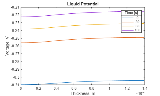
To see more details of the liquid potential distribution, plot it separately. Use the same four solution times.
figure
for i = [1 4 7 11]
plot(results.Mesh.Nodes, ...
results.LiquidPotential(i,:))
    hold on
end
title("Liquid Potential")
xlabel("Thickness, m")
ylabel("Voltage, V")
lgd = legend(num2str(results.SolutionTimes([1;4;7;11])));
lgd.Title.String = "Time [s]";
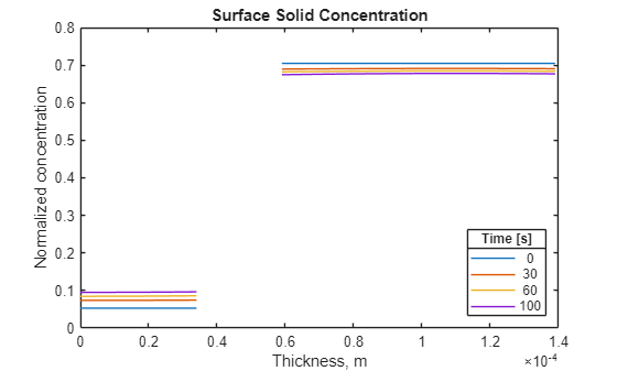
Plot the surface solid concentration distribution for the same four solution times.
figure
for i = [1 4 7 11]
plot(results.Mesh.Nodes, ...
results.SurfaceSolidConcentration(i,:))
    hold on
end
title("Surface Solid Concentration")
xlabel("Thickness, m")
ylabel("Normalized concentration")
lgd = legend(num2str(results.SolutionTimes([1;4;7;11])));
lgd.Location = "southeast";
lgd.Title.String = "Time [s]";
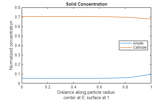
For the final solution time, 100s, plot the solid concentration along the particle radius at two locations corresponding approximately to the middle of the anode and the middle of the cathode.
figure
Rfinal = results.SolidConcentration(end,:,:);
Nr = size(results.SolidConcentration,2);
for x = [results.Mesh.AnodeNodes(ceil(end/2)) ...
         results.Mesh.CathodeNodes(ceil(end/2))]
    Rr = Rfinal(:,:,x);
plot((0:Nr-1).'/(Nr-1),Rr(:))
    hold on
end
title("Solid Concentration")
xlabel({"Distance along particle radius:";"center at 0, surface at 1"})
ylabel("Normalized concentration")
legend("Anode","Cathode",Location="east");
Input Arguments
Output Arguments
Tips
When you use modal analysis results to solve a transient structural dynamics model, the
modalresultsargument must be created in Partial Differential Equation Toolbox™ from R2019a or newer.For a frequency response model with damping, the results are complex. Use functions such as
absandangleto obtain real-valued results, such as the magnitude and phase.