Main Content

linearize

Linearize structural or thermal model

Since R2021b

Description

example

sys = linearize(model) extracts a sparse linear model for use with Control System Toolbox™. For a structural analysis model, linearize extracts a mechss (Control System Toolbox) model. For a thermal analysis model, it extracts a sparss (Control System Toolbox) model. For transient models, linearize uses time 0.

Use linearizeInput to specify the inputs of the linear model that correspond to external forcing, such as loads or internal heat sources. The toolbox treats the value of each selected constraint, load, or source as a constant, and the value becomes one input channel in the linearized model. The remaining boundary conditions are set to zero for linearization purposes, regardless of their value in the structural or thermal model. Ensure that you label all nonzero boundary conditions and pass them as inputs using linearizeInput.

Use linearizeOutput to specify the outputs of the linear model in terms of regions of the geometry, such as cells (for 3-D geometries only), faces, edges, or vertices. This includes all degrees of freedom (DoFs) in the specified region as output values. For structural models, you can also specify which of the x, y, and z degrees of freedom to include as outputs.

Use sys.InputName and sys.OutputGroup to locate the inputs and outputs of sys that correspond to a particular boundary condition or to a selected region.

example

mx = linearize(model,"OutputType","matrices") returns the finite element matrices A, B, C, D, E or M, K, B, F used to construct the mechss and sparss models in the previous syntax.

Examples

collapse all

Linearize a model for thermal analysis and return finite element matrices.

Create a transient thermal model.

thermalmodel = createpde("thermal","transient");

Add the block geometry to the thermal model by using the geometryFromEdges function. The geometry description file for this problem is called crackg.m.

geometryFromEdges(thermalmodel,@crackg);

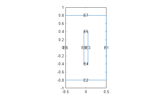
Plot the geometry with the edge labels.

pdegplot(thermalmodel,"EdgeLabels","on")
ylim([-1,1])
axis equal

Figure contains an axes object. The axes object contains 9 objects of type line, text.

Generate a mesh.

generateMesh(thermalmodel);

Specify the thermal conductivity, mass density, and specific heat of the material.

thermalProperties(thermalmodel,"ThermalConductivity",1, ...
                               "MassDensity",1, ...
                               "SpecificHeat",1);

Specify the temperature on the left edge as 100, and constant heat flow to the exterior through the right edge as -10. Add a unique label to each boundary condition.

thermalBC(thermalmodel,"Edge",6,"Temperature",100,"Label","TempBC");
thermalBC(thermalmodel,"Edge",1,"HeatFlux",-10,"Label","FluxBC");

Specify that the entire geometry generates heat and add a unique label to this assignment.

internalHeatSource(thermalmodel,25,"Label","HeatSource");

Set an initial value of 0 for the temperature.

thermalIC(thermalmodel,0);

Specify the inputs of the linearized model by calling the linearizeInput function with the previously defined labels for the boundary conditions and the internal heat source. Add one label per function call.

linearizeInput(thermalmodel,"HeatSource");
linearizeInput(thermalmodel,"TempBC");
linearizeInput(thermalmodel,"FluxBC");

Specify the outputs of the linearized model by calling the linearizeOutput function to set the regions of interest for measuring temperature. Specify one region per function call. For example, specify that the output is the temperature value at all nodes on edge 2.

linearizeOutput(thermalmodel,"Edge",2);

Measure the temperature on edge 2.

sys = linearize(thermalmodel)
Sparse continuous-time state-space model with 27 outputs, 3 inputs, and 1351 states.

Use "spy" and "showStateInfo" to inspect model structure. 
Type "help sparssOptions" for available solver options for this model.

In the linearized model, use sys.InputName to check that the inputs to sys are the heat source, the temperature on edge 6, and the heat flux on edge 1.

sys.InputName
ans = 3x1 cell
    {'HeatSource'}
    {'TempBC'    }
    {'FluxBC'    }

In the linearized model, use sys.OutputGroup to locate the sections associated with each coordinate.

sys.OutputGroup
ans = struct with fields:
    Edge2: [1 2 3 4 5 6 7 8 9 10 11 12 13 14 15 16 17 18 19 20 21 22 23 24 25 26 27]

If you do not have Control System Toolbox™, you can access the finite element matrices A, B, C, and E as follows.

mx = linearize(thermalmodel,"OutputType","matrices")
mx = struct with fields:
    A: [1351x1351 double]
    B: [1351x3 double]
    C: [27x1351 double]
    E: [1351x1351 double]

Linearize a structural model and return finite element matrices.

Create a structural transient analysis model.

structuralmodel = createpde("structural","transient-solid");

Import and plot the tuning fork geometry.

importGeometry(structuralmodel,"TuningFork.stl");
pdegplot(structuralmodel)

Figure contains an axes object. The axes object contains 6 objects of type quiver, text, patch, line.

Generate a mesh.

generateMesh(structuralmodel,"Hmax",0.005);

Specify Young's modulus, Poisson's ratio, and the mass density to model linear elastic material behavior. Specify all physical properties in consistent units.

structuralProperties(structuralmodel,"YoungsModulus",210E9, ...
                                     "PoissonsRatio",0.3, ...
                                     "MassDensity",8000);

Identify faces for applying boundary constraints and loads by plotting the geometry with the face labels.

figure("units","normalized","outerposition",[0 0 1 1])
pdegplot(structuralmodel,"FaceLabels","on")
view(-50,15)
title("Geometry with Face Labels")

Figure contains an axes object. The axes object with title Geometry with Face Labels contains 6 objects of type quiver, text, patch, line.

Impose sufficient boundary constraints to prevent rigid body motion under applied loading. Typically, you hold a tuning fork by hand or mount it on a table. A simplified approximation to this boundary condition is fixing a region near the intersection of tines and the handle (faces 21 and 22).

structuralBC(structuralmodel,"Face",[21,22],"Constraint","fixed");

Specify the pressure loading on a tine as a short rectangular pressure pulse.

structuralBoundaryLoad(structuralmodel,"Face",11,"Pressure",5E6, ...
                                       "EndTime",1e-3,"Label","Pressure");

Specify acceleration due to gravity as a body load.

structuralBodyLoad(structuralmodel,"GravitationalAcceleration",[0 0 -1], ...
                                   "Label","Gravity");

Create inputs for gravity and the pressure pulse on tuning fork.

linearizeInput(structuralmodel,"Gravity");
linearizeInput(structuralmodel,"Pressure");

Measure the y-displacement of face 12 and x-displacement of face 6.

linearizeOutput(structuralmodel,"Face",12,"Component","y");
linearizeOutput(structuralmodel,"Face",6,"Component","x");

Obtain a mechss model of the tuning fork.

sys = linearize(structuralmodel)
Sparse continuous-time second-order model with 28 outputs, 4 inputs, and 4926 degrees of freedom.

Use "spy" and "showStateInfo" to inspect model structure. 
Type "help mechssOptions" for available solver options for this model.

In the linearized model, use sys.InputName to check that the inputs to sys are the gravity body load and the pressure pulse on a tine. The gravity body load produces three inputs because it has x-, y-, and z-components.

sys.InputName
ans = 4x1 cell
    {'Gravity_x'}
    {'Gravity_y'}
    {'Gravity_z'}
    {'Pressure' }

In the linearized model, use sys.OutputGroup to locate the sections associated with each coordinate.

sys.OutputGroup
ans = struct with fields:
    Face12_y: [1 2 3 4 5 6 7 8 9 10 11 12 13]
     Face6_x: [14 15 16 17 18 19 20 21 22 23 24 25 26 27 28]

If you do not have Control System Toolbox™, you can access the finite element matrices M, K, B, and F as follows.

mx = linearize(structuralmodel,"OutputType","matrices")
mx = struct with fields:
    M: [4926x4926 double]
    K: [4926x4926 double]
    B: [4926x4 double]
    F: [28x4926 double]

Input Arguments

collapse all

Structural or thermal model, specified as a StructuralModel object or a ThermalModel object. The linearize function does not support nonlinear thermal analysis.

Example: thermalmodel = createpde("thermal","steadystate")

Example: structuralmodel = createpde("structural","static-solid")

Output Arguments

collapse all

Sparse linear models for use with Control System Toolbox, returned as a mechss or sparss model object.

Finite element matrices A, B, C, D, and E or M, K, B, and F, returned as a structure array.

Version History

Introduced in R2021b