AlphaBetaFilter
Alpha-beta filter for object tracking
Description
The AlphaBetaFilter object represents an alpha-beta filter
designed for object tracking. Use this tracker for platforms that follow a linear motion model
and have a linear measurement model. Linear motion is defined by constant velocity or constant
acceleration. Use the filter to predict the future location of an object, to reduce noise for
a detected location, or to help associate multiple objects with their tracks.
Creation
Description
abf = AlphaBetaFilterMotionModel property to
'2D Constant Velocity'. In this case, the filter state takes the
form [x; vx; y; vy].
abf = AlphaBetaFilter(Name,Value,...)Name,Value
pair arguments. Any unspecified properties take default values.
Properties
Object Functions
predict | Predict the state and state estimation error covariance |
correct | Correct the state and state estimation error covariance |
distance | Distances between measurements and predicted measurements |
likelihood | Likelihood of measurement |
clone | Create identical object |
Examples
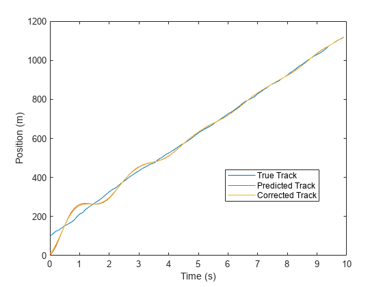
Track Constant-Velocity Target Using Alpha-Beta Filter
Apply the alpha-beta filter to track a target moving at constant velocity along the x-axis.
T = 0.1;
V0 = 100;
N = 100;
plat = phased.Platform('MotionModel','Velocity', ...
    'VelocitySource','Input port','InitialPosition',[100;0;0]);
abfilt = phased.AlphaBetaFilter('MotionModel','1D Constant Velocity');
Z = zeros(1,N);
Zp = zeros(1,N);
Zc = zeros(1,N);
for m = 1:N
    pos = plat(T,[100+20*randn;0;0]);
    Z(m) = pos(1);
    [~,~,Zp(m)] = predict(abfilt,T);
    [~,~,Zc(m)] = correct(abfilt,Z(m));
end
t = (0:N-1)*T;
plot(t,Z,t,Zp,t,Zc)
xlabel('Time (s)')
ylabel('Position (m)')
legend('True Track','Predicted Track','Corrected Track', ...
    'Location','Best')
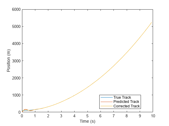
Track Constant-Acceleration Target Using Alpha-Beta Filter
Apply the alpha-beta filter to track a target moving at constant acceleration along the x-axis.
T = 0.1;
a0 = 100;
N = 100;
plat = phased.Platform('MotionModel','Acceleration', ...
    'AccelerationSource','Input port','InitialPosition',[100;0;0]);
abfilt = phased.AlphaBetaFilter( ...
    'MotionModel','1D Constant Acceleration', ...
    'Coefficients',[0.5 0.5 0.1]);
Z = zeros(1,N);
Zp = zeros(1,N);
Zc = zeros(1,N);
for m = 1:N
    pos = plat(T,[100+20*randn;0;0]);
    Z(m) = pos(1);
    [~,~,Zp(m)] = predict(abfilt,T);
    [~,~,Zc(m)] = correct(abfilt,Z(m));
end
t = (0:N-1)*T;
plot(t,Z,t,Zp,t,Zc)
xlabel('Time (s)')
ylabel('Position (m)');
legend('True Track','Predicted Track','Corrected Track', ...
    'Location','Best');
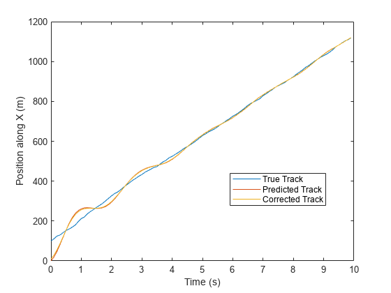
Track Target in 3-D Using Alpha-Beta Filter
Apply the alpha-beta filter to track a target moving at constant velocity in three dimensions.
T = 0.1;
V0 = 100;
N = 100;
plat = phased.Platform('MotionModel','Velocity', ...
    'VelocitySource','Input port','InitialPosition',[100;0;0]);
abfilt = phased.AlphaBetaFilter('MotionModel', ...
    '3D Constant Velocity','State',zeros(6,1));
Z = zeros(3,N);
Zp = zeros(3,N);
Zc = zeros(3,N);
for m = 1:N
    Z(:,m) = plat(T,[V0+20*randn;0;0]);
    [~,~,Zp(:,m)] = predict(abfilt,T);
    [~,~,Zc(:,m)] = correct(abfilt,Z(:,m));
end
t = (0:N-1)*T;
plot(t,Z(1,:),t,Zp(1,:),t,Zc(1,:))
xlabel('Time (s)')
ylabel('Position along X (m)')
legend('True Track','Predicted Track','Corrected Track', ...
    'Location','Best')
Extended Capabilities
Version History
Introduced in R2018b
You can also select a web site from the following list:
Americas
- América Latina (Español)
- Canada (English)
- United States (English)
Europe
- Belgium (English)
- Denmark (English)
- Deutschland (Deutsch)
- España (Español)
- Finland (English)
- France (Français)
- Ireland (English)
- Italia (Italiano)
- Luxembourg (English)
- Netherlands (English)
- Norway (English)
- Österreich (Deutsch)
- Portugal (English)
- Sweden (English)
- Switzerland
- United Kingdom (English)