Direct Signal Interference (DSI) Suppression In Passive Radar

Since R2026a

Introduction

Passive radar systems rely on opportunistic transmissions, such as broadcast television, to detect and track targets without emitting their own energy. These systems offer significant advantages in terms of stealth, cost, and spectral efficiency. However, they face a unique challenge: the received signal from a target is often many orders of magnitude weaker than the direct signal interference (DSI) which comes directly from the transmitter and clutter environment.

Effective suppression of the DSI is critical to the performance of passive radar. If not mitigated, the DSI raises the noise floor in the range-Doppler map and can obscure target returns. Several digital signal processing techniques have been developed to address this, particularly time-domain filtering approaches that estimate and subtract the DSI component using a clean reference signal.

This example investigates the performance of several such DSI suppression algorithms using simulated data in MATLAB. First we investigate the impact of signal quality and hardware impairments on the performance of a common DSI suppression algorithm, and then we compare multiple relevant DSI suppression algorithms in terms of suppression capability and runtime in static and dynamic clutter environments. The algorithms and methodology presented in this example are based on the work by Garry, Baker, and Smith [1].

Passive Radar System Overview

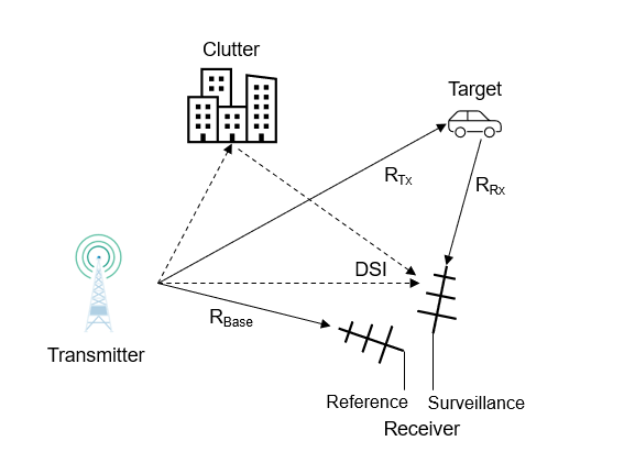
A typical passive radar system consists of two primary channels: a reference and surveillance channel:

• The reference channel receives a direct copy of the signal transmitted by the illuminator of opportunity (e.g., a broadcast tower). This signal is typically collected using a directional antenna pointed at the transmitter, resulting in a high signal-to-noise ratio (SNR).

• The surveillance channel receives echoes of the transmitted signal reflected off objects in the environment, including both potential targets and interference sources such as buildings, terrain, or the direct path signal entering the antenna's sidelobes. The surveillance signal is typically collected using a highly directional antenna pointed or steered away from the transmitter to minimize interference from the direct path.

An illustration of a typical passive radar system is shown below:

The signal entering the reference channel is modeled as:

$$s_{\text{ref}}=s_{\text{dir},\text{ref}}+n_{\text{ref}}$$

where:

• $s_{\text{dir},\text{ref}}$ is the direct path received by the reference channel

• $n_{\text{ref}}$ is the receiver noise in the reference channel

The signal entering the surveillance channel is modeled as:

$$s_{\text{surv}}=s_{\text{dsi}}+s_{\text{target}}+n_{\text{surv}}$$

where:

• $s_{\text{dsi}}$ contains both the direct path and clutter received by the surveillance channel

• $s_{\text{target}}$ is the target reflection that we are interested in detecting

• $n_{\text{surv}}$ is the receiver noise in the surveillance channel

Because the direct and multi-path interference components are often tens of decibels stronger than the desired target signals, they dominate the surveillance waveform and define the noise floor in the resulting range-Doppler (RD) map. This makes it extremely challenging to detect weak targets without first removing the dominant interference.

To address this, passive radar systems employ DSI suppression algorithms. These algorithms estimate the interference component based on the known reference signal and subtract it from the surveillance signal. Effective suppression can significantly reduce the interference power, improving the system's sensitivity and dynamic range.

Overview of DSI Suppression Algorithms

In passive radar, DSI suppression is performed according to the following graphic:

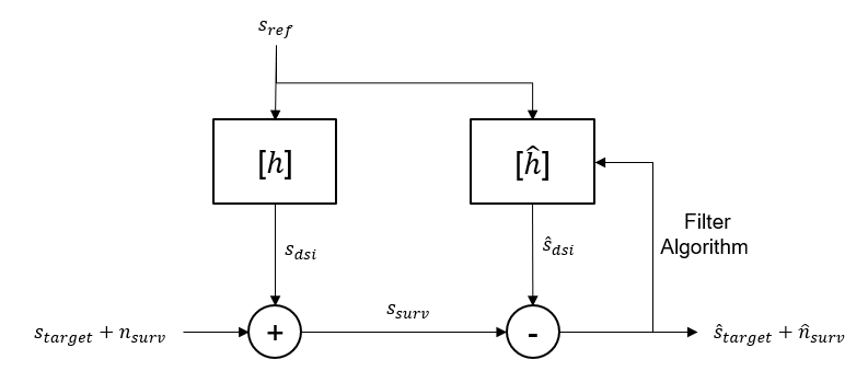
The reference signal ($s_{\text{ref}}$) is used as a proxy for the direct path signal despite containing some receiver noise. The assumed model is that $s_{\text{ref}}$ passes through the surveillance channel ($h$, made up of complex channel coefficients), to give the DSI signal ($s_{\text{dsi}}$). The DSI signal combines with the target signal ($s_{\text{target}}$) and the surveillance noise ($n_{\text{surv}}$) to give the surveillance signal ($s_{\text{surv}}$) that is measured in our surveillance channel.

In parallel, the $s_{\text{ref}}$ is passed through an estimate of the surveillance channel coefficients ($\underset{}{\overset{ˆ}{h}}$) to give an estimate of the DSI signal (${\underset{}{\overset{ˆ}{s}}}_{\text{dsi}}$). Finally, ${\underset{}{\overset{ˆ}{s}}}_{\text{dsi}}$ is subtracted from $s_{\text{surv}}$ to give an estimate of our target signal (${\underset{}{\overset{ˆ}{s}}}_{\text{target}}$) and noise (${\underset{}{\overset{ˆ}{n}}}_{\text{ref}}$).

The goal of the DSI suppression algorithms discussed in this example is to estimate the surveillance channel so that we can recover the target signal.

There are two broad categories of suppression algorithms:

• Fixed-coefficient methods, such as the Wiener-Hopf method, compute a single set of filter coefficients that remain constant over the entire coherent processing interval (CPI). These methods are computationally efficient, but may under-perform in dynamic environments where the interference characteristics change over time.

• Adaptive filtering methods, such as the least mean squares (LMS) method, update the filter coefficients either continuously or in blocks during the CPI. This allows the filter to track changes in clutter or interference over time. However, adaptive filters can also risk canceling parts of the target signal if the Doppler separation is insufficient.

The algorithms evaluated in this example include:

• Wiener-Hopf: A classical method that estimates the filter coefficients to minimize the mean squared error between the surveillance signal and the filtered reference signal. It is simple and efficient but is only effective in stationary interference environments.

• Enhanced Cancellation Algorithm by Carrier and Doppler Shift (ECA-CD): A fixed-coefficient method that enhances the least-squares formulation by projecting the surveillance signal into the orthogonal subspace of Doppler-shifted versions of the reference signal. This improves suppression of both direct path and stationary clutter, based on the approach described in [3].

• Block LMS: An adaptive algorithm that updates filter coefficients in blocks for improved performance over LMS. It provides stronger suppression performance in dynamic clutter environments than fixed-coefficient methods.

For more information on the implementation of these and other adaptive filtering techniques, see [1], [2], [3].

Signal Generation and Analysis for Testing

Before implementing any adaptive filtering algorithms, we discuss how signals are generated and how suppression is evaluated. For the eventual comparison of various clutter suppression algorithms, we will test each algorithm in both a static and dynamic clutter environment.

Signal Generation

To evaluate the performance of DSI suppression algorithms, we generate synthetic reference and surveillance channel signals that capture the essential characteristics of a passive radar system while allowing us to control parameters such as SNR and interference-to-noise ratio (INR).

The signal generation consists of the following components:

• Direct Path Signal: A bandlimited white Gaussian noise signal with random phase and amplitude is used to represent the transmitted waveform from the illuminator of opportunity.

• Reference Signal: Direct path signal plus noise at a specified SNR.

• Surveillance Channel: The surveillance channel is modeled as a tapped-delay line, where each tap represents a delayed and scaled copy of the direct path signal. The tap amplitudes are generated as complex Gaussian random variables with a power decay profile that mimics typical propagation loss of 1/$R^4$. We investigate results using both a static and dynamic clutter environment.

• Surveillance Signal: Formed by convolving the direct path signal with the surveillance channel to get the DSI signal, plus adding noise at a specified INR. No target echoes are included in this example, as the goal is to isolate and evaluate DSI suppression performance.

Static Surveillance Channel

The following code demonstrates how we generate each of these signal components for testing the suppression algorithms. Here we demonstrate signal generation when the surveillance channel is static.

rng("default");

Use 100,000 samples to create the initial signals.

nSamples = 1e5;

The direct path has random phase and amplitude.

powDir = 1;
sdir = sqrt(powDir)*randn(nSamples,1,like=1i);

The reference signal is the direct path signal with noise added.

snrRef = 80;
sref = awgn(sdir,snrRef,powDir);

We set the number of taps in the surveillance channel. The coefficients are complex Gaussian random variables. The first tap is the direct path signal which should have a power level proportional to $\frac{1}{R^2}$, whereas ensuing taps represent reflections of the direct path with objects in the environment and should have a power level proportional to $\frac{1}{R^4}$. So, the relative power of each tap with respect to the first tap should have a $\frac{1}{R^2}$ relationship. We use this notion to set the power of the taps as a function of sample index.

nTaps = 100;
rIdx = (1:nTaps)';
coeffPow = (1./rIdx).^2;
dsicoeff = sqrt(coeffPow).*randn(nTaps,1,like=1i);

The DSI signal is the direct path signal filtered through DSI channel coefficients.

sdsi = filter(dsicoeff,1,sdir);

A target signal is created with a delay of half the number of channel taps, and a normalized Doppler shift of $-\frac{2\pi }{4}$. The target is set to be 20 dB lower power than the direct path signal. Typically, the target would be even lower power. However in this example we use the target power level to measure the signal-to-interference-plus-noise ratio (SINR) before and after suppression, so we elect to use a relatively high power target to make this measurement more consistent. This is explained in more detail in the following section.

powTar = powDir/db2pow(20);
tDelay = round(nTaps/2);
tDop = -1/4;
samples = 0:nSamples-1;
starget = sqrt(powTar)*circshift(sdir,tDelay).*exp(1i*2*pi*samples'*tDop);

The surveillance signal is the DSI signal combined with the target signal and noise.

inrSurv = 80;
ssurv = sdsi + awgn(starget,inrSurv,rms(sdsi)^2);

The process for creating signals in a dynamic surveillance channel is explained briefly in the next section.

Dynamic Surveillance Channel

Later in the example, we test the DSI suppression algorithms using both static and dynamic surveillance channel coefficients. The steps for generating the dynamic surveillance channel are largely the same as the steps shown above. The major difference is that instead of applying a single set of surveillance channel taps for the entire signal duration, the taps change slightly at each time step. Depending on the passive radar environment, a dynamic surveillance channel may be a more realistic model in which to test DSI suppression algorithms.

Suppression Measurement Methodology

In order to analyze the degree of suppression achieved, we perform range-Doppler processing using the reference channel as the matched filter and measure how much the SINR is increased after DSI suppression. The sidelobe region of the range-Doppler map is used to estimate the interference plus noise power and the range-Doppler cell containing the target response is used to estimate the signal power.

To demonstrate this, we first perform range-Doppler processing using the signals generated in the prior section.

normDop = ((0:100)-50)/100;
[resp,delay] = helperBistaticRangeDoppler(ssurv,sref,nTaps,normDop);

We plot the range-Doppler response, and highlight the region that will be used to calculate the noise power in our signals.

delayNoiseRegion = [nTaps/10 nTaps-nTaps/10];
normDopNoiseRegion = [0.05 0.45];
helperPlotBistaticRangeDoppler(resp,delay,delayNoiseRegion,normDop,normDopNoiseRegion);

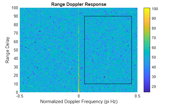
The power in the black region will be used to measure the noise in the signal before and after DSI suppression. To ensure that the suppression algorithm is not lowering both the noise and target power, we will use the signal power in the delay-Doppler bin of the target to represent our signal power.

The following plot zooms in on the target location and shows the bin that will be used to characterize signal power.

helperPlotTargetRangeDoppler(resp,delay,delayNoiseRegion,tDelay,normDop,normDopNoiseRegion,tDop);

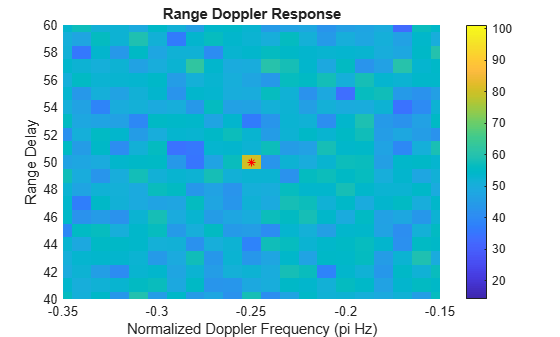
The red asterisk shows the target location.

We use the Wiener-Hopf filter to demonstrate the DSI suppression measurement technique used in this example.

First the SINR prior to suppression is measured.

sinrBefore = helperGetTargetSinr(ssurv,sref,nTaps,delayNoiseRegion,tDelay,normDop,normDopNoiseRegion,tDop);

Then, the Wiener-Hopf filter is applied.

ssurvSuppress = helperWienerHopfFilter(ssurv,sref,nTaps);

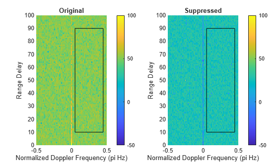
The range-Doppler response before and after suppression is plotted to show the reduction in the noise floor.

helperPlotRangeDopplerSuppression(ssurv,ssurvSuppress,sref,nTaps,delayNoiseRegion,normDop,normDopNoiseRegion);

Finally, we compute the SINR after suppression.

sinrAfter = helperGetTargetSinr(ssurvSuppress,sref,nTaps,delayNoiseRegion,tDelay,normDop,normDopNoiseRegion,tDop);
disp(['SINR increased by ',num2str(sinrAfter-sinrBefore),' dB']);

SINR increased by 22.6977 dB

This technique is used for the remainder of the example to measure the effectiveness of the DSI suppression algorithms.

Impact of Reference SNR and Surveillance INR

The performance of DSI suppression algorithms in passive radar is governed by the quality of both the reference and surveillance channels. Two key parameters define this quality:

• Reference SNR: The signal-to-noise ratio in the reference channel, which determines how accurately the transmitted waveform can be represented and used in the suppression process.

• Surveillance INR: The interference-to-noise ratio in the surveillance channel, which reflects how dominant the DSI is relative to thermal noise.

To study their effects, we apply the Wiener-Hopf filter to synthetic data while systematically varying reference SNR and surveillance INR. For each case, suppression is measured according to the procedure described in the previous section. In this section we continue to use the DSI channel coefficients generated in the prior section.

First we create the baseline surveillance signal to test varying reference channel SNR and the baseline reference signal to test varying surveillance channel INR. Both of these signals are noise free.

% Create the baseline signals
ssurvNoNoise = sdsi + starget;
srefNoNoise = sdir;

Next, we loop through varying levels of noise in the surveillance signal and reference signal. For each noise level, we estimate the effectiveness of the DSI suppression algorithm.

% Capture SNR improvement at varying noise levels
pNoise = -10:10:100;
nNoise = length(pNoise);

% Initialize the SINR increase as a function of reference SNR
refSnrSinrIncrease = zeros(nNoise,1);

% Initialize the SINR increase as a function of surveillance INR
survInrSinrIncrease = zeros(nNoise,1);

for iNoise = 1:nNoise

Capture the SINR increase as a function of reference SNR using the noiseless surveillance signal.

% Generate reference channel signal
srefNoise = awgn(sdir,pNoise(iNoise),rms(sdir)^2);

% Compute power in the range-Doppler response region of interest
sinrBefore = helperGetTargetSinr(ssurvNoNoise,srefNoise,nTaps,delayNoiseRegion,tDelay,normDop,normDopNoiseRegion,tDop);

% Perform least squares DSI suppression using Wiener-Hopf
ssurvSuppress = helperWienerHopfFilter(ssurvNoNoise,srefNoise,nTaps);

% Compute power in the range-Doppler response region
sinrAfter = helperGetTargetSinr(ssurvSuppress,srefNoise,nTaps,delayNoiseRegion,tDelay,normDop,normDopNoiseRegion,tDop);

% Save suppression
refSnrSinrIncrease(iNoise) = sinrAfter-sinrBefore;

Capture the SINR increase as a function of surveillance INR using the noiseless reference signal.

% Generate surveillance channel signal
ssurvNoise = sdsi + awgn(starget,pNoise(iNoise),rms(sdsi)^2);

% Compute power in the range-Doppler response region of interest
sinrBefore = helperGetTargetSinr(ssurvNoise,srefNoNoise,nTaps,delayNoiseRegion,tDelay,normDop,normDopNoiseRegion,tDop);

% Perform least squares DSI suppression using Wiener-Hopf
ssurvSuppress = helperWienerHopfFilter(ssurvNoise,srefNoNoise,nTaps);

% Compute power in the range-Doppler response region
sinrAfter = helperGetTargetSinr(ssurvSuppress,srefNoNoise,nTaps,delayNoiseRegion,tDelay,normDop,normDopNoiseRegion,tDop);

% Save suppression
survInrSinrIncrease(iNoise) = sinrAfter-sinrBefore;
end

Plot the DSI suppression results when varying the reference SNR and surveillance INR.

helperPlotRefSNRSurvINR(pNoise,refSnrSinrIncrease,survInrSinrIncrease);

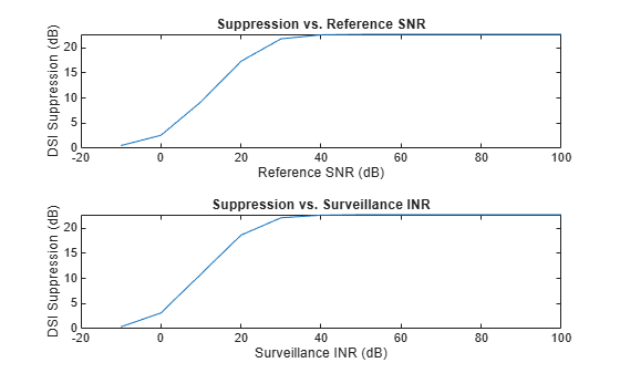
The plots above demonstrate that noise in the reference or surveillance channel has a very similar impact on the effectiveness of DSI suppression. Noise in either channel makes it more difficult to obtain an accurate channel estimate, and sets a lower limit on how much the DSI sidelobes can be suppressed until they are no longer above the noise floor.

Another interesting observation about this analysis is that there is an upper limit, regardless of noise power in either channel, on the amount of DSI suppression that is available. This upper limit exists because even without any noise or interference present in either signal, the measured noise power is limited by the sidelobes of the target response. We can demonstrate this by calculating the SINR using our described method when no noise or interference is present. We do this by setting our reference signal to the direct path signal without noise and the surveillance signal to the target signal without noise.

baseRef = sdir;
baseSurv = starget;
baseSinr = helperGetTargetSinr(baseSurv,baseRef,nTaps,delayNoiseRegion,tDelay,normDop,normDopNoiseRegion,tDop);
disp(['Maximum SINR is  ',num2str(baseSinr),' dB']);

Maximum SINR is  49.9163 dB

Therefore, no matter how little noise is present and how much the DSI is suppressed, this baseline SINR due to target sidelobes places an upper limit on the available DSI suppression with the presented measurement technique.

Impact of Hardware Impairments

While DSI suppression algorithms can be highly effective under ideal hardware conditions, real-world RF front-end impairments can significantly influence their performance. These impairments affect different parts of the passive radar chain in different ways, and their impact must be carefully considered in system modeling, system design, and signal processing.

Transmitter Impairments

Impairments to the transmit waveform—such as nonlinear distortion, phase noise, or modulation artifacts—are generally less critical in a passive setup where the receiver collects a direct-path reference signal. Since the reference channel captures the actual transmitted waveform, any distortion is inherently included in the model used for suppression.

However, this assumption breaks down if the transmit impairments significantly alter the received power level. For instance, a severe carrier frequency drift may cause the transmitted signal to fall outside the expected bandwidth of the receiver's filters, thereby reducing the received power. In such cases, even though the reference channel captures the waveform, the received target power may be lower than anticipated.

Receiver Impairments

Receive-side impairments are more critical to consider and can be divided into two broad categories: uncorrelated and correlated impairments between the reference and surveillance channel.

Uncorrelated Impairments

Uncorrelated impairments differ between the reference and surveillance channels and can have substantial impact on effectiveness of DSI suppression algorithms. One example of a type of uncorrelated impairment is thermal noise, which was already shown to have a substantial impact on DSI suppression in the prior section.

Another example of an uncorrelated impairment is nonlinearity. Nonlinear effects in the receiver RF path have greater impact on higher power signals, meaning that the reference channel may be distorted to a greater extent than the surveillance channel, impacting effectiveness of DSI suppression. This effect is demonstrated below.

Consider the case where the receiver contains a low-noise amplifier (LNA) with nonlinear behavior with input power saturation of 70 dBm.

ipsatDbm = 70;
lna = rf.Amplifier(Model='cubic',Gain=20,Nonlinearity='IPsat',IPsat=ipsatDbm,IncludeNoise=true);

Two cases are considered, one in which the reference signal is at the saturation power level of the amplifier, and another in which the reference signal is well below the saturation power level of the amplifier. The surveillance channel signal power remains well below the saturation power level of the amplifier.

pSurvDbm = ipsatDbm-40;
ampSurv = db2mag(pSurvDbm-30);
pRefLowDbm = ipsatDbm-20;
ampRefLow = db2mag(pRefLowDbm-30);
pRefHighDbm = ipsatDbm;
ampRefHigh = db2mag(pRefHighDbm-30);

The reference and surveillance signals are created at these power levels and passed through the LNA.

sdsi = filter(dsicoeff,1,sdir);
ssurv = lna(sdsi*ampSurv/rms(sdsi)+starget);
srefLow = lna(sdir*ampRefLow/rms(sdir));
srefHigh = lna(sdir*ampRefHigh/rms(sdir));

The SINR improvement when the reference channel is distorted by receiver non-linearity is compared to the case when no nonlinear distortion occurs. First the SINR prior to any filtering is measured.

sinrBefore = helperGetTargetSinr(ssurv,sdir,nTaps,delayNoiseRegion,tDelay,normDop,normDopNoiseRegion,tDop);

Then the Wiener-Hopf filter is used with the low power reference signal that has limited distortion and the high power reference that is significantly distorted.

ssurvFilterLowRef = helperWienerHopfFilter(ssurv,srefLow,nTaps);
sinrFilterLowRef = helperGetTargetSinr(ssurvFilterLowRef,sdir,nTaps,delayNoiseRegion,tDelay,normDop,normDopNoiseRegion,tDop);
disp(['SINR increased by ',num2str(sinrFilterLowRef-sinrBefore),' dB when reference channel is undistorted']);

SINR increased by 19.8058 dB when reference channel is undistorted

ssurvFilterHighRef = helperWienerHopfFilter(ssurv,srefHigh,nTaps);
sinrFilterHighRef = helperGetTargetSinr(ssurvFilterHighRef,sdir,nTaps,delayNoiseRegion,tDelay,normDop,normDopNoiseRegion,tDop);
disp(['SINR increased by ',num2str(sinrFilterHighRef-sinrBefore),' dB when reference channel is distorted']);

SINR increased by 9.7134 dB when reference channel is distorted

As expected, the effectiveness of DSI suppression is reduced due to uncorrelated distortion between channels. Therefore, it is critical to consider any uncorrelated impairments in passive radar system modeling.

Correlated Impairments

Correlated impairments impact the reference and surveillance channel equally. These kinds of impairments can still impact DSI suppression algorithms as the effect of the impairment changes over time, but the impact of such impairments is reduced compared to the impact observed for uncorrelated impairments.

One example of a correlated impairment is phase noise introduced by a local oscillator shared between the reference and surveillance channel. This can be modelled using the rf.Mixer. Two mixers are created, one with a low level of phase noise, and one with a much higher level of phase noise.

mixLowPn = rf.Mixer(IncludePhaseNoise=true,PhaseNoiseLevel=[-145 -150],SampleRate=30e6,PhaseNoiseAutoResolution=false,PhaseNoiseNumSamples=2^7,PhaseNoiseSeedSource="user",PhaseNoiseSeed=0);
mixHighPn = rf.Mixer(IncludePhaseNoise=true,PhaseNoiseLevel=[-100 -120],SampleRate=30e6,PhaseNoiseAutoResolution=false,PhaseNoiseNumSamples=2^7,PhaseNoiseSeedSource="user",PhaseNoiseSeed=0);

We create correlated phase noise between the reference and surveillance channel with both the low power phase noise and high power phase noise mixer.

smixLow = mixLowPn([ssurv,srefLow]);
smixHigh = mixHighPn([ssurv,srefLow]);

Plot the phase noise in the surveillance channel when using the low and high phase noise mixer.

helperPlotSurvPhaseNoise(smixLow,smixHigh,ssurv);

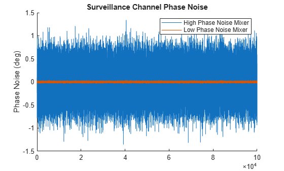
The phase noise due to the high phase noise mixer is substantially greater than the phase noise due to the low phase noise mixer.

We again calculate the SINR improvement after DSI suppression in both cases using the Wiener-Hopf filter.

ssurvLowPn = smixLow(:,1);
srefLowPn = smixLow(:,2);
sinrLowPn = helperGetTargetSinr(ssurvLowPn,srefLowPn,nTaps,delayNoiseRegion,tDelay,normDop,normDopNoiseRegion,tDop);
ssurvLowPnFilter = helperWienerHopfFilter(ssurvLowPn,srefLowPn,nTaps);
sinrLowPnFilter = helperGetTargetSinr(ssurvLowPnFilter,srefLowPn,nTaps,delayNoiseRegion,tDelay,normDop,normDopNoiseRegion,tDop);
disp(['SINR increased by ',num2str(sinrLowPnFilter-sinrLowPn),' dB when phase noise is low']);

SINR increased by 19.8057 dB when phase noise is low

ssurvHighPn = smixHigh(:,1);
srefHighPn = smixHigh(:,2);
sinrHighPn = helperGetTargetSinr(ssurvHighPn,srefHighPn,nTaps,delayNoiseRegion,tDelay,normDop,normDopNoiseRegion,tDop);
ssurvHighPnFilter = helperWienerHopfFilter(ssurvHighPn,srefHighPn,nTaps);
sinrHighPnFilter = helperGetTargetSinr(ssurvHighPnFilter,srefHighPn,nTaps,delayNoiseRegion,tDelay,normDop,normDopNoiseRegion,tDop);
disp(['SINR increased by ',num2str(sinrHighPnFilter-sinrHighPn),' dB when phase noise is high']);

SINR increased by 19.8 dB when phase noise is high

In this case, the DSI suppression algorithm is just as effective even when the phase noise is increased substantially, due to the correlation of phase noise between reference and surveillance channel. This analysis suggests modeling correlated impairments when investigating passive radars using a two-channel approach is less critical than modeling uncorrelated impairments.

Comparison of DSI Suppression Algorithms

In this section, we compare the performance of the four DSI suppression algorithms discussed earlier:

• Wiener-Hopf

• ECA-CD

• BLMS

Each algorithm is evaluated on the same simulated datasets.

Two key metrics are used to compare the algorithms:

1. Suppression performance: Measure SINR improvement using the technique described previously.

2. Runtime: Measured as the elapsed processing time in MATLAB for the full CPI. This gives a sense of the computational cost and practical feasibility of each method.

Comparisons between algorithms are made in a static environment with fixed surveillance channel coefficients and a dynamic environment with changing surveillance channel coefficients. Below we initialize waveform properties for both the static and dynamic channel environment.

rng("default");
nSamples = 1e6;
nTaps = 100;
powDir = 1;
powTar = powDir/db2pow(20);
tDelay = round(nTaps/2);
tDop = -1/4;
snrRef = 80;
inrSurv = 80;
normDop = ((0:100)-50)/100;
delayNoiseRegion = [nTaps/10 nTaps-nTaps/10];
normDopNoiseRegion = [0.05 0.45];

We then generate the reference and surveillance signals with static and dynamic surveillance channel coefficients.

[srefStatic,ssurvStatic] = helperCreateStaticChannelSignals(nSamples,nTaps,powDir,powTar,snrRef,inrSurv,tDelay,tDop);
[srefDynamic,ssurvDynamic] = helperCreateDynamicChannelSignals(nSamples,nTaps,powDir,powTar,snrRef,inrSurv,tDelay,tDop);

Measure the SINR before applying any of the suppression algorithms.

sinrInitStatic = helperGetTargetSinr(ssurvStatic,srefStatic,nTaps,delayNoiseRegion,tDelay,normDop,normDopNoiseRegion,tDop);
sinrInitDynamic = helperGetTargetSinr(ssurvDynamic,srefDynamic,nTaps,delayNoiseRegion,tDelay,normDop,normDopNoiseRegion,tDop);

Capture the Wiener-Hopf filter statistics with static and dynamic channel coefficients.

% Setup filter function
whFcn = @(ssurv,sref,nTaps)helperWienerHopfFilter(ssurv,sref,nTaps);

% Capture statistics
[whStaticSuppression,whStaticTime] = helperMeasureFilterSuppression(whFcn,sinrInitStatic,srefStatic,ssurvStatic,nTaps,delayNoiseRegion,tDelay,normDop,normDopNoiseRegion,tDop);
[whDynamicSuppression,whDynamicTime] = helperMeasureFilterSuppression(whFcn,sinrInitDynamic,srefDynamic,ssurvDynamic,nTaps,delayNoiseRegion,tDelay,normDop,normDopNoiseRegion,tDop);

Next, capture the ECA-CD filter statistics with static and dynamic channel coefficients.

% Setup filter function
dopplerColumns = 10;
dopplerColumnsCancel = 2;
ecacdFcn = @(ssurv,sref,nTaps)helperEcaCd(ssurv,sref,dopplerColumnsCancel,dopplerColumns);

% Capture statistics
[ecacdStaticSuppression,ecacdStaticTime] = helperMeasureFilterSuppression(ecacdFcn,sinrInitStatic,srefStatic,ssurvStatic,nTaps,delayNoiseRegion,tDelay,normDop,normDopNoiseRegion,tDop);
[ecacdDynamicSuppression,ecacdDynamicTime] = helperMeasureFilterSuppression(ecacdFcn,sinrInitDynamic,srefDynamic,ssurvDynamic,nTaps,delayNoiseRegion,tDelay,normDop,normDopNoiseRegion,tDop);

Finally, capture the BLMS filter statistics with static and dynamic channel coefficients. The step size is set to converge appropriately. The filter coefficients are initialized using the Wiener-Hopf approach to emulate a situation in which there is some starting estimate of the channel coefficients from previous data collections. Adaptive filters may fail to converge depending on parameter settings, so these setup steps are critical.

% Setup shared filter characteristics
blockSize = nTaps*10;
covSize = 1e3;

% Setup the filter for the static channel
cov = (ssurvStatic(1:covSize)*ssurvStatic(1:covSize)')/covSize;
stepSize = 1/(2*blockSize*max(eig(cov)));
[~,hinit] = helperWienerHopfFilter(srefStatic,ssurvStatic,nTaps);
filt = dsp.BlockLMSFilter(Length=nTaps,BlockSize=blockSize,StepSize=stepSize,InitialWeights=hinit);
staticFiltFcn = @(ssurv,sref,nTaps)helperExecuteBLMS(filt,ssurv,sref);

% Setup the filter for the dynamic channel
cov = (ssurvDynamic(1:covSize)*ssurvDynamic(1:covSize)')/covSize;
stepSize = 1/(2*blockSize*max(eig(cov)));
[~,hinit] = helperWienerHopfFilter(srefDynamic,ssurvDynamic,nTaps);
filt = dsp.BlockLMSFilter(Length=nTaps,BlockSize=blockSize,StepSize=stepSize,InitialWeights=hinit);
dynamicFiltFcn = @(ssurv,sref,nTaps)helperExecuteBLMS(filt,ssurv,sref);

% Capture statistics
[blmsStaticSuppression,blmsStaticTime] = helperMeasureFilterSuppression(staticFiltFcn,sinrInitStatic,srefStatic,ssurvStatic,nTaps,delayNoiseRegion,tDelay,normDop,normDopNoiseRegion,tDop);
[blmsDynamicSuppression,blmsDynamicTime] = helperMeasureFilterSuppression(dynamicFiltFcn,sinrInitDynamic,srefDynamic,ssurvDynamic,nTaps,delayNoiseRegion,tDelay,normDop,normDopNoiseRegion,tDop);

The statistics for each filter are compared for the static and dynamic surveillance channel coefficients.

Below is a comparison of the filter statistics with static surveillance channel coefficients.

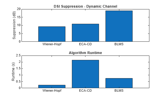
algSuppression = [whStaticSuppression,ecacdStaticSuppression,blmsStaticSuppression];
algTime = [whStaticTime,ecacdStaticTime,blmsStaticTime];
algNames = ["Wiener-Hopf","ECA-CD","BLMS"];
helperCompareSuppression(algSuppression,algTime,algNames,'Static Channel');

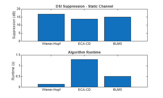
In the static surveillance channel, the fixed coefficient method (Wiener-Hopf) is fast and has the best suppression performance. ECA-CD and BLMS are slower and do not perform as well as the static coefficient methods.

The strength of adaptive filtering methods are demonstrated when the channel coefficients are dynamic, as shown in the plot below.

algSuppression = [whDynamicSuppression,ecacdDynamicSuppression,blmsDynamicSuppression];
algTime = [whDynamicTime,ecacdDynamicTime,blmsDynamicTime];
algNames = ["Wiener-Hopf","ECA-CD","BLMS"];
helperCompareSuppression(algSuppression,algTime,algNames,'Dynamic Channel');

In the dynamic surveillance channel, BLMS has the best suppression results. Therefore, depending on the clutter environment that your system is operating in, an adaptive coefficient method such as BLMS may be preferable despite some trade-off in runtime.

Conclusion

This example demonstrates the effectiveness of several DSI suppression algorithms in a simulated passive radar scenario. We examined how noise and hardware impairments in the reference and surveillance channels impact suppression performance. Three suppression algorithms—Wiener-Hopf, ECA-CD, and BLMS—were evaluated in terms of suppression performance and runtime in both a static and dynamic clutter environment. Fixed coefficient algorithms like Wiener-Hopf perform best under the static channel coefficient assumption, whereas the BLMS filter performed best in the presence of dynamic channel coefficients. Ultimately, the best DSI suppression algorithm will be dependent on the clutter environment and should be evaluated on a case-by-case basis.

References

1. Garry, Joseph Landon, Chris J. Baker, and Graeme E. Smith. "Evaluation of direct signal suppression for passive radar." IEEE Transactions on Geoscience and Remote Sensing 55, no. 7 (2017): 3786-3799.

2. Palmer, James E., and Stephen J. Searle. "Evaluation of adaptive filter algorithms for clutter cancellation in passive bistatic radar." In 2012 IEEE Radar conference, pp. 0493-0498. IEEE, 2012.

3. Schwark, Christoph, and Diego Cristallini. "Advanced multipath clutter cancellation in OFDM-based passive radar systems." In 2016 IEEE Radar Conference (RadarConf), pp. 1-4. IEEE, 2016.

Helper Functions

function [resp,delay] = helperBistaticRangeDoppler(surv,ref,nLag,normFreq)
    % Perform range-Doppler processing by correlating Doppler shifted
    % versions of the reference waveform with the surveillance waveform for
    % nLags.

    % Get the sample delays
    delay = -nLag:nLag;
    
    % Cross correlate each surveillance with Doppler shifted reference
    nFreq = length(normFreq);
    samples = (0:(length(surv)-1))';
    resp = zeros(length(delay),nFreq);
    for iCol = 1:nFreq
        refShift = ref.*exp(1i*2*pi*normFreq(iCol)*samples);
        resp(:,iCol) = abs(xcorr(surv,refShift,nLag));
    end
end

function helperPlotBistaticRangeDoppler(resp,delay,delayNoiseRegion,normDop,normDopNoiseRegion,ax)
    arguments
        resp
        delay
        delayNoiseRegion
        normDop
        normDopNoiseRegion
        ax = axes(figure)
    end

    % Plot the image, only show positive delays
    delayKeep = delay >= 0;
    delayPlot = delay(delayKeep);
    hold(ax,"on");
    imagesc(ax,normDop,delayPlot,mag2db(resp(delayKeep,:)));
    title(ax,'Range Doppler Response');
    xlabel(ax,'Normalized Doppler Frequency (pi Hz)');
    ylabel(ax,'Range Delay');
    ax.YDir = 'normal';
    colorbar(ax);

    % Plot the range-angle region being measured
    delStart = delayNoiseRegion(1);
    delStop = delayNoiseRegion(2);
    dopStart = normDopNoiseRegion(1);
    dopStop = normDopNoiseRegion(2);
    plot(ax,[dopStart dopStart],[delStart delStop],Color='k');
    plot(ax,[dopStop dopStop],[delStart delStop],Color='k');
    plot(ax,[dopStart dopStop],[delStart delStart],Color='k');
    plot(ax,[dopStart dopStop],[delStop delStop],Color='k');

    % Set lims
    xlim(ax,[normDop(1) normDop(end)]);
    ylim(ax,[delayPlot(1) delayPlot(end)]);
end

function helperPlotTargetRangeDoppler(resp,delay,delayNoiseRegion,tDelay,normDop,normDopNoiseRegion,tDop)
    % Zoom in on the target region in the range-Doppler response.
    tarAx = axes(figure);
    helperPlotBistaticRangeDoppler(resp,delay,delayNoiseRegion,normDop,normDopNoiseRegion,tarAx);
    xlim(tarAx,[tDop-0.1 tDop+0.1]);
    ylim(tarAx,[tDelay-10 tDelay+10]);
    scatter(tarAx,tDop,tDelay,"red",Marker="*");
end

function helperPlotRangeDopplerSuppression(ssurv,ssurvSuppress,sref,nTaps,delayNoiseRegion,normDop,normDopNoiseRegion)
    % Setup axes
    f = figure;
    tl = tiledlayout(f,"horizontal");
    nsAx = nexttile(tl);
    sAx = nexttile(tl);

    % Get response without suppression
    [respNoSuppress,delay] = helperBistaticRangeDoppler(ssurv,sref,nTaps,normDop);
    helperPlotBistaticRangeDoppler(respNoSuppress,delay,delayNoiseRegion,normDop,normDopNoiseRegion,nsAx);

    % Get response with suppression
    [respSuppress,delay] = helperBistaticRangeDoppler(ssurvSuppress,sref,nTaps,normDop);
    helperPlotBistaticRangeDoppler(respSuppress,delay,delayNoiseRegion,normDop,normDopNoiseRegion,sAx);

    % Update charts
    nsAx.Title.String = 'Original';
    sAx.Title.String = 'Suppressed';
    nsAx.CLim = [-50 100];
    sAx.CLim = [-50 100];
end

function helperPlotRefSNRSurvINR(pNoise,refSnrSinrIncrease,survInrSinrIncrease)
    % Plot the impact of reference SNR and surveillance INR on the DSI
    % suppression algorithm.
    
    % Create axes
    tl = tiledlayout(figure,"vertical");
    axRefSNR = nexttile(tl);
    axSurvINR = nexttile(tl);

    % Plot suppression as a function of reference SNR
    plot(axRefSNR,pNoise,refSnrSinrIncrease);
    xlabel(axRefSNR,'Reference SNR (dB)');
    ylabel(axRefSNR,'DSI Suppression (dB)');
    title(axRefSNR,'Suppression vs. Reference SNR');

    % Plot suppression as a function of surveillance INR
    plot(axSurvINR,pNoise,survInrSinrIncrease);
    xlabel(axSurvINR,'Surveillance INR (dB)');
    ylabel(axSurvINR,'DSI Suppression (dB)');
    title(axSurvINR,'Suppression vs. Surveillance INR');
end

function powDb = helperGetTargetSinr(ssurv,sref,nTaps,delayNoiseRegion,tDelay,normDop,normDopNoiseRegion,tDop)
    % Compute range-Doppler
    [resp,delay] = helperBistaticRangeDoppler(ssurv,sref,nTaps,normDop);

    % Get the response in the target region to measure signal
    [~,tDelayIdx] = min(abs(delay-tDelay));
    [~,tDopIdx] = min(abs(normDop-tDop));
    tResp = resp(tDelayIdx,tDopIdx);

    % Get the response in the region of interest to measure noise
    delStart = delayNoiseRegion(1);
    delStop = delayNoiseRegion(2);
    keepDelay = delay >= delStart & delay <= delStop;
    dopStart = normDopNoiseRegion(1);
    dopStop = normDopNoiseRegion(2);
    keepDop = normDop >= dopStart & normDop <= dopStop;
    noiseResp = resp(keepDelay,keepDop);

    % Calulate the power in the response area of interest
    tarPow = abs(tResp)^2;
    noisePow = rms(noiseResp,"all").^2;
    powDb = pow2db(tarPow/noisePow);
end

function [sref,ssurv,sdir,dsicoeff] = helperCreateStaticChannelSignals(nSamples,nTaps,powDir,powTar,snrRef,inrSurv,tDelay,tDop)
    % Create initial signals and static dsi coefficients
    [sdir,sref,dsicoeff] = helperCreateInitSignals(nSamples,powDir,snrRef,nTaps);
    
    % DSI signal is the direct path filtered through DSI channel
    sdsi = filter(dsicoeff,1,sdir);
    
    % Create target signal
    samples = 0:nSamples-1;
    starget = sqrt(powTar)*circshift(sdir,tDelay).*exp(1i*2*pi*samples'*tDop);
    
    % Create the surveillance signal
    ssurv = sdsi + awgn(starget,inrSurv,rms(sdsi)^2);
end

function [sref,ssurv] = helperCreateDynamicChannelSignals(nSamples,nTaps,powDir,powTar,snrRef,inrSurv,tDelay,tDop)
    % Create signals when DSI channel is dynamic.

    % Create initial signals and static dsi coefficients
    [sdir,sref,dsicoeffInit] = helperCreateInitSignals(nSamples,powDir,snrRef,nTaps);
    dsicoeff = dsicoeffInit;

    % For each time step, apply some small variation to the channel
    % coefficients. The amount that we change on each step could be
    % adjusted based on the use case.
    changeMag = 1e-4;
    sdsi = zeros(nSamples,1);
    for iSample = 1:nSamples
        % Filter just the current sample

        % Get the current filter length
        endSample = min(iSample+nTaps-1,nSamples);
        nFiltSamples = endSample-iSample+1;
        
        % Store current sample to pass through filter
        cSample = zeros(nFiltSamples,1);
        cSample(1) = sdir(iSample);

        % Filter current samples through dynamic DSI coefficients
        cSurv = filter(dsicoeff,1,cSample);
        sdsi(iSample:endSample) = sdsi(iSample:endSample) + cSurv;
        
        % Randomly update DSI coefficients
        dsiChange = changeMag * randn(nTaps,1,like=1i);
        dsicoeffNew = dsicoeff + dsiChange;

        % Normalize so that the total channel power doesn't change
        dsicoeff = dsicoeffNew * sqrt((dsicoeff'*dsicoeff)/(dsicoeffNew'*dsicoeffNew));
    end
    
    % Create target signal
    samples = 0:nSamples-1;
    starget = sqrt(powTar)*circshift(sdir,tDelay).*exp(1i*2*pi*samples'*tDop);
    
    % Create the surveillance signal
    ssurv = sdsi + awgn(starget,inrSurv,rms(sdsi)^2);
end

function [sdir,sref,dsicoeff] = helperCreateInitSignals(nSamples,powDir,snrRef,nTaps)
    % Create the direct path signal, ref signal, and static DSI coefficients
    
    % Direct path has random phase and amplitude
    sdir = sqrt(powDir)*randn(nSamples,1,like=1i);
    
    % Reference signal is the direct path with noise added.
    sref = awgn(sdir,snrRef,powDir);
    
    % Surveillance channel coefficients have random phase and ampitude
    % decreasing with 1/R^2 relative to first tap.
    rIdx = (1:nTaps)';
    coeffPow = (1./rIdx).^2;
    dsicoeff = sqrt(coeffPow).*randn(nTaps,1,like=1i);
end

function [survest,h] = helperWienerHopfFilter(surv,ref,M)
    % Compute autocorrelation and cross-correlation with conjugates
    rxx = xcorr(ref, M-1, 'biased');
    rsx = xcorr(surv, ref, M-1, 'biased');
    
    % Extract centered values (zero lag at index M)
    Rxx = toeplitz(rxx(M:end));
    rsx_vec = conj(rsx(M:end));
    
    % Solve Wiener-Hopf equation
    h = conj(Rxx \ rsx_vec);
    
    % Remove the filtered reference from surveillance
    survest = surv - filter(h,1,ref);
end

function [x,ref] = helperEcaCd(surv,ref,nCancelBins,nPulse)
    % Rearrange the surveillance and reference channel into nPulses. Clip
    % the input data to fit nPulses.
    ns = length(surv);
    nSamplePerPulse = floor(ns/nPulse);
    ns = nSamplePerPulse*nPulse;
    surv = surv(1:ns);
    ref = ref(1:ns);
    survMat = reshape(surv,[nSamplePerPulse nPulse]);
    refMat = reshape(ref,[nSamplePerPulse nPulse]);
    
    % Convert time-domain signal in frequency domain
    X = fft(survMat,[],1);
    Xref = fft(refMat,[],1);
    
    % Doppler spread matrix
    dopres = 1/nPulse;
    dopSpreadMatrix = dopsteeringvec((-nCancelBins*dopres:dopres:nCancelBins*dopres),nPulse);
    
    % Interference mitigation in slow-time
    Xcancel = zeros(nSamplePerPulse,nPulse);
    for iSample = 1:nSamplePerPulse
        % Signals over slow-time
        xRefSlow = Xref(iSample,:).';
        xSlow = X(iSample,:).';
    
        % If interference has Doppler spread, consider these spreaded Doppler
        % for interference nulling
        xRefSlow = dopSpreadMatrix.*xRefSlow;
    
        % Projection matrix onto the interference subspace
        projectMatrix = xRefSlow/(xRefSlow'*xRefSlow)*xRefSlow';
    
        % Cancel interference 
        Xcancel(iSample,:) = xSlow - projectMatrix*xSlow;
    end
    
    % Convert signal back to time-domain
    x = ifft(Xcancel);
    x = reshape(x,[ns 1]);
end

function suppressionDb = helperCompareSuppression(suppressionDb,algTimes,algNames,infoStr)
    % Create a tiled layout - one tile for suppression, one for run time.
    f = figure;
    tl = tiledlayout(f);
    axSuppress = nexttile(tl);
    axTime = nexttile(tl);

    % Plot suppression
    bar(axSuppress,algNames,suppressionDb);
    title(axSuppress,['DSI Suppression - ',infoStr]);
    ylabel(axSuppress,"Suppression (dB)");

    % Plot runtime
    bar(axTime,algNames,algTimes);
    title(axTime,"Algorithm Runtime");
    ylabel(axTime,"Runtime (s)");
end

function helperPlotSurvPhaseNoise(smixLow,smixHigh,ssurv)
    % Plot phase noise in the surveillance channel
    ax = axes(figure);
    hold(ax,"on");
    plot(ax,rad2deg(angle(smixHigh(:,1)./ssurv)),DisplayName='High Phase Noise Mixer');
    plot(ax,rad2deg(angle(smixLow(:,1)./ssurv)),DisplayName='Low Phase Noise Mixer');
    title(ax,'Surveillance Channel Phase Noise');
    ylabel(ax,'Phase Noise (deg)');
    legend(ax);
end

function [suppression,exTime] = helperMeasureFilterSuppression(fcn,sinrInit,sref,ssurv,nTaps,delayNoiseRegion,tDelay,normDop,normDopNoiseRegion,tDop)
    % Measure the suppression and the execution time for the given filter
    % fcn.
    ssurvSuppress = fcn(ssurv,sref,nTaps);
    sinrFinal = helperGetTargetSinr(ssurvSuppress,sref,nTaps,delayNoiseRegion,tDelay,normDop,normDopNoiseRegion,tDop);
    suppression = sinrFinal-sinrInit;
    exTime = timeit(@()fcn(ssurv,sref,nTaps));
end

function survSuppress = helperExecuteBLMS(filt,ssurv,sref)
    % Use filt to suppress sref in ssurv.
    [~,survSuppress] = filt(sref,ssurv);
end