Simulating Radar Systems with Atmospheric Refraction
The performance of a radar system is closely tied to the environment in which it operates. This example will discuss one of the environmental factors that is outside of the system designer's control, namely the atmosphere. This example will focus on refraction effects due to the atmosphere and its impact on target parameter estimation. As a part of this example, two different sensor types, one a waveform-level sensor that produces IQ and the other a statistical measurement-level sensor that produces detections, will be presented to show how to work at different levels of abstraction and how the two sensors produce similar results when configured appropriately.
This example demonstrates errors due to refraction for an L-band surveillance radar operating at a mid latitude during winter. It first configures a radar scenario and reviews built-in atmospheric models available in Radar Toolbox™. Next it presents a simple exponential approximation for the refractivity versus height. It then uses these models to generate IQ using a waveform-level sensor radarTransceiver and processes the IQ to generate detections. A measurement-level sensor radarDataGenerator is then configured based on the radarTransceiver settings to produce statistical detections to demonstrate working at a higher level of abstraction. Lastly, detections from radarTransceiver and radarDataGenerator are used in an analysis showing refraction errors for the specified scenario geometry and how the errors match predictions.
Define Radar Parameters
Define an L-band monostatic surveillance radar that has coherent processing intervals (CPIs) that are 64 pulses long. The sensor is a stationary system mounted to a tower 10 meters above the surface.
% Set random number generator to ensure results are repeatable
rng('default')

% Sensor parameters
freq       = 2e9;  % L-band center frequency (Hz)
numPulses  = 64;   % Number of pulses in a CPI
prf        = 4e3;  % PRF (Hz)
tpd        = 1e-5; % Pulse width (s)
fs         = 3e7;  % Sampling frequency (Hz)
bw         = fs/2; % Bandwidth (Hz)
sensorHgt  = 10;   % Sensor height above the surface (m)
Given the bandwidth, determine the range resolution using the bw2rangeres function.
bw2rangeres(bw) % Range resolution (m)ans = 9.9931
Configure the Radar Scenario
First configure the target positions for the analysis. Within this scenario, 15 different target positions will be considered. Set the target elevation angles to a constant 3 degrees with true slant ranges (also called the geometric range) varying from 1 to 30 km. Set the target radar cross section (RCS) to 10 dBsm, which is representative of a large aircraft.
% Target parameters
numTgtPos  = 15;                             % Target positions
tgtRCSdBsm = 10;                             % Target RCS (dBsm)
tgtEl      = 3;                              % Target elevation (deg)
tgtSR      = linspace(1,30,numTgtPos)*1e3;   % Target slant range (m)
tgtSpeed   = 90;                             % Target speed (m/s)
updateTime = (tgtSR(2) - tgtSR(1))/tgtSpeed; % Update time (sec)
Calculate the flight duration and create a radar scenario.
flightDuration = (numTgtPos - 1).*updateTime;
updateRate = 1/updateTime;
scene = radarScenario('UpdateRate',updateRate, ...
    'IsEarthCentered',true,'StopTime',flightDuration);
Add the Atmosphere
Simulating the refraction phenomenon requires a model of the atmosphere. For this example, the built-in atmospheres available in the refractiveidx function will be used. The refractiveidx function offers six ITU reference atmospheric models, namely:
Standard atmospheric model, also known as the Mean Annual Global Reference Atmosphere (MAGRA)
Summer high latitude model (higher than 45 degrees)
Winter high latitude model (higher than 45 degrees)
Summer mid latitude model (between 22 and 45 degrees)
Winter mid latitude model (between 22 and 45 degrees)
Low latitude model (smaller than 22 degrees)
Select the mid latitude model in winter. More information about these atmospheric models can be found in the Modeling Target Position Errors Due to Refraction example.
The Central Radio Propagation Laboratory (CRPL) developed a widely used reference atmosphere model that approximates the refractivity profile as an exponential decay versus height. In general, the CRPL model is a good approximation for refractivity profiles under normal propagation conditions. This exponential decay model underlies the CRPL method in the following functions:
height2rangeheight2grndrangerange2heightslant2rangerefractionexp
It also exists as an atmosphere option within a radar scenario.
The CRPL exponential model is given by
where is the surface refractivity (N-units), is the height (km), and is a decay constant (1/km) calculated as
.
In the above equation, is the difference between the surface refractivity and the refractivity at a height of 1 km. can be approximated by an exponential function expressed as
.
The CRPL exponential model is easily modified to match local conditions by setting appropriate surface refractivity and refractive exponent values. Use the surface refractivity output from the refractiveidx function as an input to the CRPL model. Calculate the decay constant (refraction exponent) using the refractionexp function.
% Define CRPL model parameters
[~,N0] = refractiveidx(0,'LatitudeModel','Mid','Season','Winter'); % Surface refractivity (N-units)
rexp   = refractionexp(N0);                                        % Corresponding refraction exponent (1/km)
Define the atmosphere model of the radar scenario as CRPL. Set the surface refractivity and refraction exponent to the previously obtained values. The selected atmosphere impacts the refraction experienced by targets in the radar scenario.
atmosphere(scene,'CRPL','SurfaceRefractivity',N0,'RefractionExponent',rexp)
ans =
  AtmosphereCRPL with properties:

    SurfaceRefractivity: 311.8587
     RefractionExponent: 0.1434
       MaxNumIterations: 10
              Tolerance: 0.0100
Configure the Waveform-Level Sensor
First define a sensor trajectory using geoTrajectory and add the trajectory to a platform.
% Surface parameters
surfHgt    = 52;  % Surface height at sensor (m)

% Setup sensor trajectory
sensoralt  = sensorHgt + surfHgt; % Surface altitude (m)
sensorpos1 = [42.30141195164364,-71.376098592854,sensoralt]; % Natick, MA USA [Lat (deg) Lon (deg) Alt (m)]
sensorpos2 = sensorpos1;
sensorTraj = geoTrajectory([sensorpos1;sensorpos2],[0;flightDuration]);

% Add sensor platform to scenario
sensorplat = platform(scene,'Trajectory',sensorTraj);
Next configure the monostatic radar sensor using radarTransceiver. This is a waveform-level model that generates IQ. Define the antenna as a rectangular phased array of size 6-by-6 with half-wavelength spacing. Set the waveform modulation to be an LFM.
% Configure radarTransceiver
[lambda,c] = freq2wavelen(freq);
elementSpacing = lambda/2;
uraSize = [6 6];
numElements = prod(uraSize);
array = phased.URA('Size',uraSize,'ElementSpacing',elementSpacing);
maxRange = 40e3;
xcvrSensor = radarTransceiver('MountingAngles',[90 0 0],'NumRepetitions',numPulses,'RangeLimits',[0 maxRange]);
xcvrSensor.Waveform = phased.LinearFMWaveform('SampleRate',fs,'PulseWidth',tpd, ...
    'PRF',prf,'SweepBandwidth',bw);
xcvrSensor.Transmitter.Gain = 15;
xcvrSensor.Receiver.Gain = 15;
xcvrSensor.Receiver.SampleRate = fs;
xcvrSensor.TransmitAntenna.Sensor = array;
xcvrSensor.ReceiveAntenna.Sensor = array;
xcvrSensor.TransmitAntenna.OperatingFrequency = freq;
xcvrSensor.ReceiveAntenna.OperatingFrequency = freq;
Attach the radarTransceiver to the sensor platform.
sensorplat.Sensors = {xcvrSensor};Define Target Trajectory
Convert target range and angle to geodetic coordinates using aer2geodetic.
% Define a structure for the target truth
tgtTruth.Range = tgtSR;
tgtTruth.Elevation = tgtEl*ones(1,numTgtPos);

% Convert azimuth, elevation, and range to geodetic positions
tgtpos     = zeros(numTgtPos,3);           % Target [lat lon alt]
tgtposTime = zeros(numTgtPos,1);           % Position times
refS       = wgs84Ellipsoid;               % Earth model
for m = 1:numTgtPos
    [tgtLat,tgtLon,tgtalts] = aer2geodetic(90,tgtEl,tgtSR(m), ...
        sensorpos1(1),sensorpos1(2),sensoralt,refS);
    tgtpos(m,:) = [tgtLat tgtLon tgtalts];
    tgtposTime(m) = (m - 1).*updateTime;
end
tgtTruth.Height = tgtpos(:,3).' - surfHgt; % Target height above the surface (m)
Define the target trajectory using geoTrajectory and attach to a target platform.
% Add target platform to scenario
tgtTraj = geoTrajectory(tgtpos,tgtposTime);
platform(scene,'Trajectory',tgtTraj,'Signature',{rcsSignature('Pattern',tgtRCSdBsm)});
Visualize the radar and target geometry by using the helper helperRadarGlobeViewer. The radar platform is shown as the blue dot and the target platform is shown as the red dot. The white line indicates the constant elevation target trajectory.
% Visualize the scenario
gv = helperRadarGlobeViewer;
showScenario(gv,scene)
positionCamera(gv,[42.1417 -71.3920 1.4668e+03],[359.9981 5.3302 31.7642])
Setup a Signal Processing Chain
In this section, the objects for a signal processing chain will be configured to process the IQ from radarTransceiver. At a high-level, the signal processing chain proceeds as depicted.

First, the simulated IQ is range and Doppler processed.
Next, the data is beamformed to broadside.
The beamformed data is then processed by a 2-dimensional constant false alarm rate detector (CFAR) to generate detections. Only the highest SNR detection is retained.
The azimuth and elevation angles of the target are then estimated using a sum/difference beamformer.
Lastly, the range of the target is further refined by quadratic interpolation. The output of this chain is the target detection.
First, configure phased.RangeDopplerResponse to create an object to perform range and Doppler processing on the simulated datacube.
% Initialize range/Doppler processing objects
matchingCoeff = getMatchedFilter(xcvrSensor.Waveform);
rngdopresp = phased.RangeDopplerResponse('OperatingFrequency',freq,'SampleRate',fs, ...
    'DopplerFFTLengthSource','Property','DopplerFFTLength',numPulses, ...
    'DopplerOutput','Speed','PRFSource','Property','PRF',prf);
Define a steering vector object that will be used to create a range-angle plot, as well as to beamform prior to performing CFAR detection.
% Beamforming
steeringvec = phased.SteeringVector('SensorArray',array);

% Create steering vector for initial range-angle visualization
elVec = -40:1:40;
sv = steeringvec(freq,[zeros(1,numel(elVec)); elVec]);
numBeams = numel(elVec);
Next, define a 2-D CFAR with 3 guard cells and 15 training cells on each side of the cell under test in range and 1 guard cell and 3 training cells in Doppler. Set the false alarm rate to 1e-6.
% 2-D CFAR
Pfa  = 1e-6; % Probability of false alarm
cfar = phased.CFARDetector2D('GuardBandSize',[3 1], ...
    'TrainingBandSize',[15 3], ...
    'ProbabilityFalseAlarm',Pfa,'OutputFormat','Detection index','NoisePowerOutputPort',true);
Define a sum/difference beamformer for angle estimation and create a range estimator object for improved range estimation.
% Angle estimation
sumdiff = phased.SumDifferenceMonopulseTracker2D('SensorArray',array,'OperatingFrequency',freq);

% Range estimation object
rangeestimator = phased.RangeEstimator;
Collect and Process IQ from the Waveform-Level Sensor
Now, advance the scenario and collect IQ from radarTransceiver using the receive method.
% Initialize simulation
numSamples = 1/prf*fs;
xcvrDets = struct('Range',zeros(1,numTgtPos), ...
    'Angles',zeros(2,numTgtPos), ...
    'SNRdB',zeros(1,numTgtPos));
hRAMplot = [];
hRDMplot = [];

% Collect and process IQ
for m = 1:numTgtPos
    % Advance scene
    advance(scene);

    % Update geometry visualization
    updateDisplay(gv,scene.SimulationTime,[scene.Platforms{:}]);

    % Collect IQ from radarTransceiver
    tmp2 = receive(scene);
Range and Doppler process the simulated IQ from radarTransceiver.
    % Range-Doppler process
    iqsig = tmp2{1};
    [resp,rngVec,dopVec] = rngdopresp(iqsig,matchingCoeff);
Next, beamform the data to get a sense of the range-angle performance.
    % Beamform across all angles
    respAng = permute(resp,[2 1 3]); % <numElements x numRange x numDoppler>
    respAng = reshape(respAng,numElements,[]); % <numElements x numRange*numDoppler>
    respAng = (sv'*respAng); % <numBeams x numRange*numDoppler>
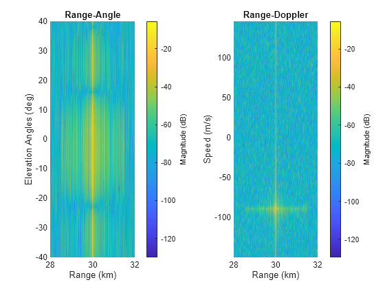
Plot the range-angle and range-Doppler data using helperPlotIQ.
    % Convert to dB and plot
    respAng = reshape(respAng,numBeams,size(iqsig,1),size(iqsig,3)); % <numBeams x numRange x numDoppler>
    respAng = permute(respAng,[2 1 3]); % <numRange x numBeams x numDoppler>
    [~,idxMax] = max(abs(respAng(:)));
    [idxMaxRange,idxMaxBeam,idxMaxDop] = ind2sub(size(respAng),idxMax);

    angRespMagdB = mag2db(squeeze(abs(respAng(:,:,idxMaxDop))));
    respMagdB = mag2db(squeeze(abs(respAng(:,idxMaxBeam,:))));

    [hRAMplot,hRDMplot] = helperPlotIQ(hRAMplot,hRDMplot, ...
        rngVec,elVec,dopVec,angRespMagdB,respMagdB,tgtSR(m));
Finally, detect and estimate the target range and angle using the helper function helperDetectAndEstimateXCVR. This helper function contains the broadside beamforming, CFAR detection, and angle and range estimation processing steps.
    % Detect targets and estimate range and angle
    xcvrDets = helperDetectAndEstimateXCVR(cfar,sumdiff,steeringvec,rangeestimator, ...
        m,rngVec,dopVec,resp,xcvrDets);
end
Configure the Measurement-Level Sensor
Define a radarDataGenerator sensor based on the radarTransceiver design above. The radarDataGenerator object is a statistical, measurement-level model that produces detections. We will compare the results from both sensor types.
% Define range, azimuth, and elevation resolutions
rangeres = bw2rangeres(bw);       % Range resolution (m)
azres    = beamwidth(array,freq); % Azimuth resolution (deg)
elres    = azres;                 % Elevation resolution (deg)

% Calculate the SNR at an arbitrary reference range
refRange = 550e3; % Reference range (m)
refRangeSNR = radareqsnr(lambda,refRange,xcvrSensor.Transmitter.PeakPower,tpd, ...
    'RCS',db2pow(tgtRCSdBsm),'Gain',[xcvrSensor.Transmitter.Gain xcvrSensor.Receiver.Gain]);
coherentProcessingGain = pow2db(numPulses);
g = beamwidth2gain([azres; elres],'IdealElliptical');
scanLoss = pow2db(cosd(tgtEl)); % Scan loss (dB)
refRangeSNR = refRangeSNR + 2*g + scanLoss + coherentProcessingGain;

% Calculate the probability of detection at the reference range
[Pd,SNR] = rocpfa(Pfa,'MinSNR',refRangeSNR - 1,'MaxSNR',refRangeSNR + 1); % ROC curve
refPd = rocinterp(SNR,Pd,refRangeSNR,'snr-pd');

% Define statistical radar
rdgSensor = radarDataGenerator(1,'UpdateRate',updateRate,'DetectionCoordinates','Sensor spherical', ...
    'MountingAngles',[90 0 0],'ScanMode','No scanning','FieldOfView',[20 20], ...
    'CenterFrequency',freq,'Bandwidth',bw,'HasNoise',false,'HasElevation',true, ...
    'AzimuthResolution',azres,'ElevationResolution',elres,'RangeResolution',rangeres, ...
    'AzimuthBiasFraction',0,'ElevationBiasFraction',0,'RangeBiasFraction',0, ...
    'ReferenceRCS',tgtRCSdBsm,'ReferenceRange',refRange,'DetectionProbability',refPd,'HasFalseAlarms',false);
Attach the radarDataGenerator to the sensor platform.
% Attach sensors
sensorplat.Sensors = {xcvrSensor,rdgSensor};
Collect Detections from the Measurement-Level Sensor
First restart the scenario. Then, advance the scenario as before, and collect detections from radarDataGenerator using the detect method.
% Restart simulation
restart(scene);

% Initialize outputs
rdgDets = struct('Range',zeros(1,numTgtPos), ...
    'Angles',zeros(2,numTgtPos), ...
    'SNRdB',zeros(1,numTgtPos));

% Gather detections
for m = 1:numTgtPos
    % Advance scene
    advance(scene);

    % Collect detections from radarDataGenerator
    tmp1 = detect(scene);
    rdgDets.Range(m) = tmp1{1}.Measurement(3);
    rdgDets.Angles(:,m) = [tmp1{1}.Measurement(1); -tmp1{1}.Measurement(2)];
    rdgDets.SNRdB(m) = tmp1{1}.ObjectAttributes{1}.SNR;
end
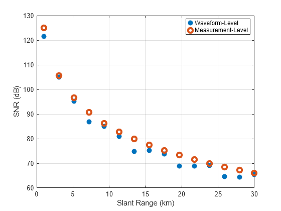
Compare the SNR of the detections from radarTransceiver and radarDataGenerator. The detections from radarTransceiver (waveform-level) are shown as blue circles, and the detections from the statistical radarDataGenerator (measurement-level) model are shown as the red circles. Overall, the measurements agree fairly well. The small differences in the SNR may be due to signal processing losses like range bin straddling or inaccuracies in estimating the direction of the target.
% SNR
co = colororder;
ax = axes(figure('Name','SNR (dB)'));
plot(ax,tgtSR*1e-3,xcvrDets.SNRdB,'o','MarkerFaceColor',co(1,:),'LineWidth',1.5)
hold(ax,'on')
grid(ax,'on')
plot(ax,tgtSR*1e-3,rdgDets.SNRdB,'o','LineWidth',3,'MarkerSize',7)
xlabel(ax,'Slant Range (km)')
ylabel(ax,'SNR (dB)')
legend(ax,'Waveform-Level','Measurement-Level','Location','Best')
Assess the Refraction Errors
Predict the range and elevation of the target along the trajectory including refraction effects. For the calculation of the predicted range and elevation angle, use the slant2range function with the CRPL method selected.
% Estimate propagated range using CRPL
[predicted.Range,predicted.Elevation,k] = slant2range( ...
    tgtTruth.Range,sensorHgt,tgtTruth.Height, ...
    'Method','CRPL','SurfaceRefractivity',N0,'RefractionExponent',rexp);
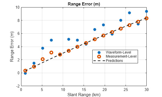
Now calculate the range error. The range error is the difference between the propagated range and the true slant range. The detected ranges match well with the predicted range errors, shown as the dashed black line in the figure. Note that the waveform-level detections are biased. This bias can be attributed to factors like:
The range resolution of the system, which is fairly large at about 10 m, and
Range bin straddling.
% Calculate the range error (m)
ax = axes(figure('Name','Range Error (m)'));
plot(ax,tgtSR*1e-3,xcvrDets.Range - tgtTruth.Range,'o','MarkerFaceColor',co(1,:),'LineWidth',1.5)
hold(ax,'on')
grid(ax,'on')
plot(ax,tgtSR*1e-3,rdgDets.Range - tgtTruth.Range,'o','LineWidth',3,'MarkerSize',7)
plot(ax,tgtSR*1e-3,predicted.Range - tgtTruth.Range,'k--','LineWidth',1.5)
xlabel(ax,'Slant Range (km)')
ylabel(ax,'Range Error (m)')
title(ax,'Range Error (m)')
legend(ax,'Waveform-Level','Measurement-Level','Predictions','Location','Best')
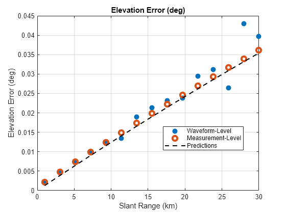
Next calculate the elevation error. The elevation error is the difference between the detected elevation angle and the true elevation angle. Note that the detected errors match the predicted elevation errors well. As the target moves farther out in range, the elevation errors increase for the waveform-level sensor due to factors like:
The effects of refraction,
Additional bias in the measurements due to the decrease in SNR, and
The increasing angular resolution with distance.
% Calculate the elevation angle error (deg)
ax = axes(figure('Name','Elevation Error (deg)'));
plot(ax,tgtSR*1e-3,xcvrDets.Angles(2,:) - tgtTruth.Elevation,'o','MarkerFaceColor',co(1,:),'LineWidth',1.5)
hold(ax,'on')
grid(ax,'on')
plot(ax,tgtSR*1e-3,rdgDets.Angles(2,:) - tgtTruth.Elevation,'o','LineWidth',3,'MarkerSize',7)
plot(ax,tgtSR*1e-3,predicted.Elevation - tgtTruth.Elevation,'k--','LineWidth',1.5)
xlabel(ax,'Slant Range (km)')
ylabel(ax,'Elevation Error (deg)')
title(ax,'Elevation Error (deg)')
legend(ax,'Waveform-Level','Measurement-Level','Predictions','Location','Best')
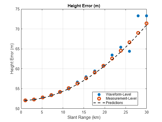
Next, calculate the height error. The height error is the difference between the apparent height, which is the height calculated assuming no refraction and the true target height. To calculate the apparent height, use the aer2geodetic function. Note that the detected height errors match the predicted height errors well. As the target moves farther out in range, the height errors slowly increase.
% Calculate apparent height from detections
[~,~,xcvrDets.Height] = aer2geodetic(90,xcvrDets.Angles(2,:),xcvrDets.Range, ...
        sensorpos1(1),sensorpos1(2),sensoralt,refS);
[~,~,rdgDets.Height] = aer2geodetic(90,rdgDets.Angles(2,:),rdgDets.Range, ...
        sensorpos1(1),sensorpos1(2),sensoralt,refS);

% Calculate apparent height from predicted path
[~,~,predicted.Height] = aer2geodetic(90,predicted.Elevation,predicted.Range, ...
        sensorpos1(1),sensorpos1(2),sensoralt,refS);

% Plot height errors (m)
ax = axes(figure('Name','Height Error (m)'));
plot(ax,tgtSR*1e-3,xcvrDets.Height - tgtTruth.Height,'o','MarkerFaceColor',co(1,:),'LineWidth',1.5)
hold(ax,'on')
grid(ax,'on')
plot(ax,tgtSR*1e-3,rdgDets.Height - tgtTruth.Height,'o','LineWidth',3,'MarkerSize',7)
plot(ax,tgtSR*1e-3,predicted.Height - tgtTruth.Height,'k--','LineWidth',1.5)
xlabel(ax,'Slant Range (km)')
ylabel(ax,'Height Error (m)')
title(ax,'Height Error (m)')
legend(ax,'Waveform-Level','Measurement-Level','Predictions','Location','Best')
Summary
This example demonstrated how to model refraction for an L-band surveillance radar operating at a mid latitude during winter at two different levels of abstraction, namely the waveform and measurement levels. Lastly, it discussed the target detection errors due to refraction and compared results to predictions.
Helpers
function [hRAMplot,hRDMplot] = helperPlotIQ(hRAMplot,hRDMplot, ...
    rngVec,elVec,dopVec,angRespMagdB,respMagdB,tgtRng)
% Plot range-angle and range-Doppler maps

if isempty(hRAMplot)
    % Initialize range-angle plot
    figure
    tiledlayout(1,2)
    nexttile
    hRAMplot = pcolor(rngVec*1e-3,elVec,angRespMagdB.');
    hRAMplot.EdgeColor = 'none';
    hRAMplot.FaceColor = 'interp';
    ylabel('Elevation Angles (deg)')
    xlabel('Range (km)')
    title('Range-Angle')
    hC = colorbar;
    hC.Label.String = 'Magnitude (dB)';

    % Initialize range-Doppler plot
    nexttile
    hRDMplot = pcolor(rngVec*1e-3,dopVec,respMagdB.');
    hRDMplot.EdgeColor = 'none';
    hRDMplot.FaceColor = 'interp';
    ylabel('Speed (m/s)')
    xlabel('Range (km)')
    title('Range-Doppler')
    hC = colorbar;
    hC.Label.String = 'Magnitude (dB)';
else
    % Update range-angle plot
    hRAMplot.CData = angRespMagdB.';

    % Update range-Doppler plot
    hRDMplot.CData = respMagdB.';
end
xlim(hRAMplot.Parent,[max((tgtRng - 2e3),rngVec(1)) min((tgtRng + 2e3),rngVec(end))]*1e-3)
xlim(hRDMplot.Parent,[max((tgtRng - 2e3),rngVec(1)) min((tgtRng + 2e3),rngVec(end))]*1e-3)
pause(0.1)
end

function xcvrDets = helperDetectAndEstimateXCVR(cfar,sumdiff,steeringvec,rangeestimator, ...
    tgtIdx,rngVec,dopVec,iqPCDP,xcvrDets)
% Detection processing. Performs the following:
% - Broadside beamforming
% - 2D CFAR
% - Angle estimation
% - Range estimation

% Number of bins
numRngBins = numel(rngVec);
numDopBins = numel(dopVec);

% Convert datacube to power
freq = sumdiff.OperatingFrequency; % Operating frequency (Hz)
sv = steeringvec(freq,[0;0]); % Broadside
iqPCDPtmp = permute(iqPCDP,[2 1 3]); % <elements x range x Doppler>
iqPCDPBF = (sv'*reshape(iqPCDPtmp,[],numRngBins*numDopBins)); % Beamform <beams x range x Doppler>
iqPow = abs(squeeze(iqPCDPBF)).^2; % Power (Watts)
iqPow = reshape(iqPow,numel(rngVec),numel(dopVec)); % Power <range x Doppler>

% Run 2D CFAR. The indices of the cells under test for the CFAR must
% permit the stencil size.
numRngStencil = cfar.GuardBandSize(1) + cfar.TrainingBandSize(1);
numDopStencil = cfar.GuardBandSize(2) + cfar.TrainingBandSize(2);
idxRngTest = (numRngStencil + 1):(numel(rngVec) - numRngStencil);
idxDopTest = (numDopStencil + 1):(numel(dopVec) - numDopStencil);
[idxRngGrid,idxDopGrid] = meshgrid(idxRngTest,idxDopTest);
[idxDet,noisePwr] = cfar(iqPow,[idxRngGrid(:).'; idxDopGrid(:).']);

% Assume maximum detection SNR is target
idxDetLinear = sub2ind(size(iqPow),idxDet(1,:),idxDet(2,:));
snrDet = iqPow(idxDetLinear)./noisePwr;
[~,idxMax] = max(snrDet);
idxRng = idxDet(1,idxMax);
idxDop = idxDet(2,idxMax);

% Estimate true angle
xcvrDets.Angles(:,tgtIdx) = sumdiff(squeeze(iqPCDP(idxRng,:,idxDop)), ...
    [0; 0]); % Estimate angle assuming sensor is aligned with target
xcvrDets.Angles(2,tgtIdx) = -xcvrDets.Angles(2,tgtIdx);

% Beamform to detected angle
sv = steeringvec(freq,xcvrDets.Angles(:,tgtIdx));
iqPCDPBF = (sv'*squeeze(iqPCDP(:,:,idxDop)).');

% Estimate SNR and range
xPower = abs(squeeze(iqPCDPBF)).^2;
xcvrDets.Range(tgtIdx) = rangeestimator(iqPCDPBF(:),rngVec,idxRng);
SNRy = pow2db(xPower((idxRng-1):(idxRng+1))./median(xPower));
rngX = rngVec((idxRng-1):(idxRng+1));
xcvrDets.SNRdB(tgtIdx) = interp1(rngX,SNRy,xcvrDets.Range(tgtIdx),'pchip');
end