Automatic Parking Valet with Unreal Engine Simulation

This example demonstrates the design of a hybrid controller for an automatic searching and parking task. You will learn how to combine adaptive model predictive control (MPC) with reinforcement learning (RL) to perform a parking maneuver. Unreal Engine® is used for environment perception and visualization.

The control objective is to park the vehicle in an empty spot after starting from an initial pose. The control algorithm executes a series of maneuvers while sensing and avoiding obstacles in tight spaces. It switches between an adaptive MPC controller and a reinforcement learning agent to complete the parking maneuver.

The adaptive MPC controller moves the vehicle at a constant speed along a reference path while searching for an empty parking spot. When a spot is found, the reinforcement learning agent takes over and executes a parking maneuver according to its pretrained policy. Prior knowledge of the environment (the parking lot) including the locations of the empty spots and parked vehicles is available to both controllers.

Parking Lot

The parking lot environment used in this example is a subsection of the Large Parking Lot (Automated Driving Toolbox) scene. The ParkingLotManager object stores information on the ego vehicle, empty parking spots, and static obstacles (parked cars and boundaries), while the ParkingLotVisualizer object creates a 2D visualization of the scene. In the 2D visualization, each parking spot has a unique index number and an indicator light that is either green (free) or red (occupied). Parked vehicles are represented in black.

Specify a sample time ${\mathit{T}}_{\mathit{s}}$ (seconds) for the controllers and a simulation time ${\mathit{T}}_{\mathit{f}}$ (seconds).

Ts = 0.1;
Tf = 50;

Create a reference path for the ego vehicle using the createReferenceTrajectory method of the ParkingLotManager object. The reference path starts from the southeast corner of the parking lot and ends at the western edge as displayed with the dashed pink line.

parkingLot = ParkingLotManager;
xRef = parkingLot.createReferenceTrajectory(Ts,Tf);
info = parkingLot.getInfo();

Set the parking space at index 18 as the free spot and fill all the other spots with static vehicle actors.

freeSpotIndex = 18;
mdl = "rlAutoParkingValet3D";
setupActorVehicles(mdl,freeSpotIndex);

Create a ParkingLotVisualizer object with a free spot at index 18 and the specified reference path xRef. Enable the visualizer figure's Visible property so that it opens outside the live script.

visualizer = ParkingLotVisualizer(freeSpotIndex,Ts,Tf);
set(gcf,Visible="on");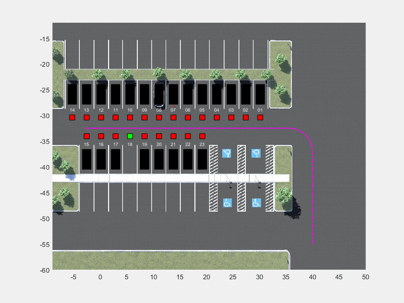

Specify an initial pose $\left({\mathit{X}}_0,{\mathit{Y}}_0,{\theta }_0\right)$ for the ego vehicle. The units of ${\mathit{X}}_0$ and ${\mathit{Y}}_0$ are meters and ${\theta }_0$ is in radians.

egoInitialPose = [40 -55 pi/2];

Compute the target pose for the vehicle using the findGoalPose method of the ParkingLotManager object. The goal pose corresponds to the location in freeSpotIdx.

vehiclePose = [10 -32.5 pi];
egoTargetPose = parkingLot.findGoalPose(vehiclePose,freeSpotIndex);

Sensor Modules

The parking algorithm uses a geometric "mode selector" object to scan for available parking spots and a lidar sensor to generate detections from the environment.

Mode Selector

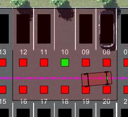
The mode selector system scans a conical area in front of the vehicle for free parking spots. The scanning area is represented by the area shaded in green in the following figure. The camera has a field of view $\phi$ bounded by $\pm$60 degrees and a maximum measurement depth ${\mathit{d}}_{\max }$ of 10 m (equal to searchDist).

searchDist = 10;

As the ego vehicle moves forward, the mode selector system senses the parking spots within the field of view and determines whether a spot is free or occupied. For simplicity, this action is implemented using geometrical relationships between the spot locations and the current vehicle pose. A parking spot is within the scanning range if ${\mathit{d}}_{\mathit{i}}\le {\mathit{d}}_{\max }$ and ${\phi }_{\min }\le {\phi }_{\mathit{i}}\le {\phi }_{\max }$, where ${\mathit{d}}_{\mathit{i}}$ is the distance to the parking spot and ${\phi }_{\mathit{i}}$ is the angle to the parking spot. Once a free parking spot is identified within the scanning area, the vehicle switches from the path-following adaptive MPC controller to the RL controller used to execute the parking maneuver.

Lidar

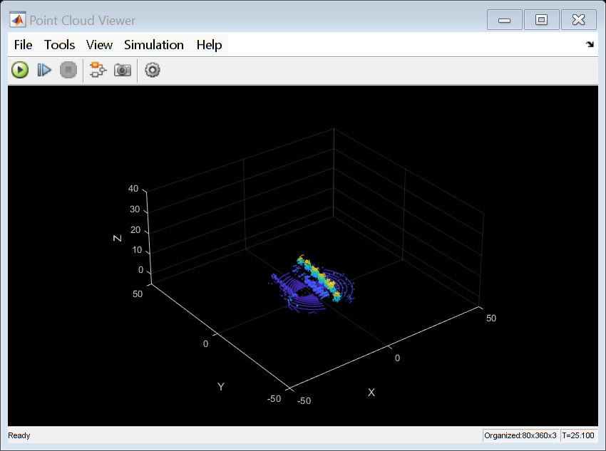
A Simulation 3D Lidar (Automated Driving Toolbox) block is used to generate a point cloud of detections from the environment. The lidar is mounted to the roof center and has a horizontal field-of-view (FOV) of 360 degrees and a vertical FOV of 40 degrees.The point cloud generated by the lidar contains five channels. The first three channels contain the $\mathit{X}$, $\mathit{Y}$, and $\mathit{Z}$ position, in meters, of each detection relative to the sensor. In the lidar sensor's coordinate system, the X-axis extends forward from the vehicle, the Y-axis extends to the left of the vehicle (as viewed when looking in the forward direction of the vehicle), and the Z-axis points up. The fourth channel of the point cloud contains the straight-line distance to each detection in meters. The fifth channel contains the reflectivity of each detection, normalized in the range [0,1]. The reinforcement learning agent uses this point cloud data to understand its environment.

Auto Parking Valet Model

Load the automatic parking valet parameters.

autoParkingValetParams3D

The parking valet model, including the controllers, ego vehicle, sensors, and parking lot, is implemented as a Simulink model. Open the model.

open_system(mdl)

In this model:

• The vehicle is modeled in the Vehicle Dynamics and Sensing subsystem. The vehicle kinematics are modeled using a single-track bicycle kinematics model with two input signals, vehicle speed $\mathit{v}$ (m/s) and steering angle $\delta$ (radians).

• The adaptive MPC and RL agent blocks are found in the MPC Tracking Controller and RL Controller subsystems, respectively.

• Mode switching between the controllers is handled by the Vehicle Mode Selector subsystem, which outputs an "isParking" signal indicating whether the vehicle is actively making a parking maneuver. Initially, the vehicle is in search mode and the adaptive MPC controller tracks the reference path. When a free spot is found, the "isParking" signal activates the RL Agent to perform the parking maneuver.

• The Unreal Engine Visualization and Sensing subsystem handles animation of the environment. You can choose to enable Unreal Engine visualization and/or 3D point cloud visualization. Double-click this subsystem to specify the visualization options.

Unreal Engine visualization can slow down the simulation, so the Enable Unreal Engine visualization parameter is automatically disabled when training the agent.

Adaptive Model Predictive Controller Design

Create the adaptive MPC controller object for reference trajectory tracking using the createMPCForParking3D script. For more information on adaptive MPC, see Adaptive MPC (Model Predictive Control Toolbox).

createMPCForParking3D;

Reinforcement Learning Controller Design

To train the reinforcement learning agent, you must create an environment interface and an agent object.

Create Environment

The environment for training is defined as a rectangular area surrounding the free parking spot, visualized by the region shaded in red in the following figure. Constraining the training to this region significantly reduces training duration when compared to training over the entire parking lot area.

The free spot selected for each training episode is randomly selected from one of four spot locations, with two on each side of the isle. This randomization is done to make the agent more robust to different vehicle shapes, sizes, colors, and lighting.

For this environment:

• The training region is a 13.625 m x 12.34 m space with the target spot at its horizontal center.

• The observations are the position errors ${\mathit{X}}_{\mathit{e}}$ and ${\mathit{Y}}_{\mathit{e}}$ of the ego vehicle with respect to the target pose, the heading angle error ${\theta }_{\mathit{e}}$, and the five-channel lidar point cloud. The position and heading error observations are scaled to the range [-1, 1] and the lidar data is scaled to the range [0, 1].

• The vehicle speed during training varies randomly between 1 and 4 m/s each episode and is held constant for the entire episode.

• The action signal is a continuous steering angle that ranges between +/- $\pi /4$ radians.

• The vehicle is considered parked if the errors with respect to target pose are within specified tolerances of +/- 0.75 m (position) and +/-10 degrees (heading).

• The episode is terminated if the ego vehicle parks successfully, leaves the training region, or collides with an obstacle.

The reward ${\mathit{r}}_{\mathit{t}}$ provided at time t, is:

$${\mathit{r}}_{\mathit{t}}=2{\mathit{e}}^{-\left(0.05{{\mathit{X}}_{\mathit{e}}}^2+0.04{{\mathit{Y}}_{\mathit{e}}}^2\right)}+0.5{\mathit{e}}^{-40{{\theta }_{\mathit{e}}}^2}-0.05{\delta }^2+100{\mathit{f}}_{\mathit{t}}-50{\mathit{g}}_{\mathit{t}}$$

Here, ${\mathit{X}}_{\mathit{e}}$, ${\mathit{Y}}_{\mathit{e}}$, and ${\theta }_{\mathit{e}}$ are the position and heading angle errors of the ego vehicle from the target pose, while $\delta$ is the steering angle. ${\mathit{f}}_{\mathit{t}}$ (0 or 1) indicates whether the vehicle has parked and ${\mathit{g}}_{\mathit{t}}$ (0 or 1) indicates if the vehicle has collided with an obstacle or left the training region at time $\mathit{t}$.

Create the observation specifications for the environment using the Simulink bus object stored in ObservationBus.mat.

load("ObservationBus.mat","ObservationBus")
obsInfo = bus2RLSpec("ObservationBus");
obsNames = [obsInfo(1).Name, obsInfo(2).Name];

Create the action specifications for the environment.

nAct = 1;
actInfo = rlNumericSpec([nAct 1],LowerLimit=-1,UpperLimit=1);
actNames = "actionInput";

Specify the path to the RL Agent block and create the Simulink environment interface. .

agentBlock = mdl + "/Controller/RL Controller/RL Agent";
env = rlSimulinkEnv(mdl,agentBlock,obsInfo,actInfo,UseFastRestart="off");

Specify a reset function for training. The autoParkingValetResetFcn3D function randomly resets the initial pose of the ego vehicle at the start of each episode.

env.ResetFcn = @autoParkingValetResetFcn3D;

For more information on creating Simulink environments, see rlSimulinkEnv.

Create Agent

The agent in this example is a twin-delayed deep deterministic policy gradient (TD3) agent. TD3 agents rely on actor and critic approximator objects to learn the optimal policy. To learn more about TD3 agents, see Twin-Delayed Deep Deterministic (TD3) Policy Gradient Agents.

The actor and critic networks are initialized randomly. Ensure reproducibility by fixing the seed of the random generator.

rng(0)

Create Critics

TD3 agents use two parameterized Q-value function approximators to estimate the value of the policy. The output of the critic network is the state-action value function for a taking a given action from a given observation.

Define each network path as an array of layer objects and assign names to the input and output layers of each path. These names allow you to connect the paths and then later explicitly associate the network input and output layers with the appropriate environment channel.

% Lidar path
lidarPath = [
    imageInputLayer(obsInfo(2).Dimension,Name="lidarData",Normalization="none")
    convolution2dLayer([5 5],8,Padding="same")
    reluLayer
    maxPooling2dLayer([3 3],Padding="same",Stride=[3 3])
    convolution2dLayer([5 5],8,Padding="same")
    reluLayer
    maxPooling2dLayer([3 3],Padding="same",Stride=[3 3])
    flattenLayer
    tanhLayer
    fullyConnectedLayer(512)
    reluLayer
    fullyConnectedLayer(256,Name="lidar_fc")];

% Pose path
posePath = [
    featureInputLayer(obsInfo(1).Dimension(1),Name="poseInfo")
    fullyConnectedLayer(64,Name="pose_fc")];

% Action path
actionInput = [
    featureInputLayer(actInfo(1).Dimension(1),Name="actionInput")
    fullyConnectedLayer(32,Name="action_fc")];

% Concatenated path
mainPath = [
    concatenationLayer(1,3,Name="concat")
    reluLayer
    fullyConnectedLayer(256)
    reluLayer
    fullyConnectedLayer(128)
    reluLayer
    fullyConnectedLayer(1,Name="criticOutLyr")];

% Convert to layerGraph object and connect layers
criticNet = layerGraph(lidarPath);
criticNet = addLayers(criticNet,posePath);
criticNet = addLayers(criticNet,actionInput);
criticNet = addLayers(criticNet,mainPath);

criticNet = connectLayers(criticNet,"lidar_fc","concat/in1");
criticNet = connectLayers(criticNet,"pose_fc","concat/in2");
criticNet = connectLayers(criticNet,"action_fc","concat/in3");

Convert to a dlnetwork object and display information about the network including the number of learnable parameters and information on the network inputs.

criticdlnet = dlnetwork(criticNet);
summary(criticdlnet)

   Initialized: true

   Number of learnables: 585.8k

   Inputs:
      1   'lidarData'     16×360×5 images
      2   'poseInfo'      3 features
      3   'actionInput'   1 features

Create the critics using criticdlnet, the environment observation and action specifications, and the names of the network input layers to be connected with the environment observation and action channels. For more information see rlQValueFunction.

critic = rlQValueFunction(criticdlnet,obsInfo,actInfo,...
    ObservationInputNames=obsNames, ActionInputNames=actNames);

Create Actors

Create the neural network for the actor. The output of the actor network is the steering angle.

% Lidar path
lidarPath = [
    imageInputLayer(obsInfo(2).Dimension,Name="lidarData",Normalization="none")
    convolution2dLayer([5 5],8,Padding="same")
    reluLayer
    maxPooling2dLayer([3 3],Padding="same",Stride=[3 3])
    convolution2dLayer([5 5],8,Padding="same")
    reluLayer
    maxPooling2dLayer([3 3],Padding="same",Stride=[3 3])
    flattenLayer
    tanhLayer
    fullyConnectedLayer(512)
    reluLayer
    fullyConnectedLayer(256,Name="lidar_fc")];

% Pose path
posePath = [
    featureInputLayer(obsInfo(1).Dimension(1),Name="poseInfo")
    fullyConnectedLayer(64,Name="pose_fc")];

% Concatenated path
mainPath = [
    concatenationLayer(1,2,Name="concat")
    reluLayer
    fullyConnectedLayer(256)
    reluLayer
    fullyConnectedLayer(128)
    reluLayer
    fullyConnectedLayer(actInfo(1).Dimension(1),Name="criticOutLyr")
    tanhLayer];

% Convert to layerGraph object and connect layers
actorNet = layerGraph(lidarPath);
actorNet = addLayers(actorNet,posePath);
actorNet = addLayers(actorNet,mainPath);

actorNet = connectLayers(actorNet,"lidar_fc","concat/in1");
actorNet = connectLayers(actorNet,"pose_fc","concat/in2");

Convert to a dlnetwork object and display information about the network.

actordlnet = dlnetwork(actorNet);
summary(actordlnet)

   Initialized: true

   Number of learnables: 577.5k

   Inputs:
      1   'lidarData'   16×360×5 images
      2   'poseInfo'    3 features

Create the actor object for the TD3 agent. For more information see rlContinuousDeterministicActor.

actor = rlContinuousDeterministicActor(actordlnet,obsInfo,actInfo);

Specify the agent options and create the TD3 agent. For more information on TD3 agent options, see rlTD3AgentOptions.

agentOpts = rlTD3AgentOptions(SampleTime=Ts, ...
    DiscountFactor=0.99, ...
    ExperienceBufferLength=1e6, ...
    MiniBatchSize=256);

Set the noise options for exploration.

agentOpts.ExplorationModel.StandardDeviation = 0.1;
agentOpts.ExplorationModel.StandardDeviationDecayRate = 1e-4;
agentOpts.ExplorationModel.StandardDeviationMin = 0.01;

For this example, set the actor and critic learn rates to 1e-3, respectively. Set a gradient threshold factor of 1 to limit the gradients during training. For more information, see rlOptimizerOptions.

Specify training options for the actor.

agentOpts.ActorOptimizerOptions.LearnRate = 1e-3;
agentOpts.ActorOptimizerOptions.GradientThreshold = 1;
agentOpts.ActorOptimizerOptions.L2RegularizationFactor = 1e-3;

Specify training options for the critic.

agentOpts.CriticOptimizerOptions(1).LearnRate = 1e-3;
agentOpts.CriticOptimizerOptions(1).GradientThreshold = 1;

Create the agent using the actor, the critics, and the agent options objects. For more information, see rlTD3Agent.

agent = rlTD3Agent(actor,critic,agentOpts);

Train Agent

To train the agent, first specify the training options.

The agent is trained for a maximum of 10000 episodes with each episode lasting a maximum of 200 time steps. The training terminates when the maximum number of episodes is reached or the average reward over 200 episodes reaches a value of 116 or greater. Specify the options for training using the rlTrainingOptions function.

trainOpts = rlTrainingOptions(...
    MaxEpisodes=10000,...
    MaxStepsPerEpisode=200,...
    ScoreAveragingWindowLength=200,...
    Plots="training-progress",...
    StopTrainingCriteria="AverageReward",...
    StopTrainingValue=116,...
    UseParallel=false);

Train the agent using the train function. Fully training this agent is a computationally intensive process that may take several hours to complete. To save time while running this example, load a pretrained agent by setting doTraining to false. To train the agent yourself, set doTraining to true.

doTraining = false;
if doTraining
    setVisualizationOptions(UEViz="off",PCViz="off"); % Disable UE and point cloud visualization
    agent = setDeviceForAgentTraining(agent); % If a GPU device is available, enable it for agent training
    trainingResult = train(agent,env,trainOpts); % Start training agent
else
    load("ParkingValetAgentTrained.mat","agent");
end

Simulate Parking Task

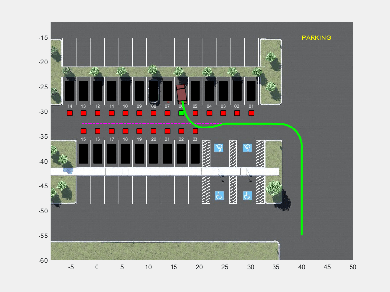
To validate the trained agent, simulate the model and observe the parking maneuver. Enable both Unreal Engine and point cloud visualization to get a more complete view of the vehicle's behavior.

setVisualizationOptions(UEViz="on",PCViz="on");
sim(mdl);

The vehicle tracks the reference path using the MPC controller before switching to the RL controller when the target spot is detected. The vehicle then completes the parking maneuver.

Change the free spot to the other side of the aisle and park the vehicle again.

freeSpotIndex = 6;
setupActorVehicles(mdl,freeSpotIndex);
sim(mdl);

To view the trajectory graphically, open the Ego Vehicle Pose scope.

open_system(mdl + "/Vehicle Dynamics and Sensing/Ego Vehicle Model/Ego Vehicle Pose")

Local Functions

function agent = setDeviceForAgentTraining(agent)
% Determine whether a GPU device is available and
% enable it for training if so.

    try gpuDevice;
        critic = getCritic(agent);
        critic(1).UseDevice = "gpu";
        setCritic(agent, critic);
    
        actor = getActor(agent);
        actor(1).UseDevice = "gpu";
        setActor(agent, actor);
    
        disp('GPU device found, using GPU for agent training.')
    catch ME
        disp('No GPU device found, using CPU for agent training.')
    end
end

function setVisualizationOptions(options)
%   This function takes two inputs, UEViz and PCViz, which enable or
%   disable Unreal Engine visualization and point cloud visualization,
%   respectively. UEViz and PCViz are both boolean scalars.
    
    arguments
        options.UEViz {mustBeTextScalar} = "on"
        options.PCViz {mustBeTextScalar} = "on"
    end


    if options.UEViz == "on"
        set_param(strcat(bdroot, "/Vehicle Dynamics and Sensing/Unreal Engine Visualization and Sensing"), ...
            enableUEViz="on");
    else
        set_param(strcat(bdroot, "/Vehicle Dynamics and Sensing/Unreal Engine Visualization and Sensing"), ...
            enableUEViz="off");
    end
    
    if options.PCViz == "on"
        set_param(strcat(bdroot, "/Vehicle Dynamics and Sensing/Unreal Engine Visualization and Sensing"), ...
            enablePCViz="on");
    else 
        set_param(strcat(bdroot, "/Vehicle Dynamics and Sensing/Unreal Engine Visualization and Sensing"), ...
            enablePCViz="off");
    end
end