Operations with RF Circuit Objects
This example shows how to create and use RF Toolbox™ circuit objects. In this example, you create three circuit (rfckt) objects: two transmission lines and an amplifier.
You visualize the amplifier data using RF Toolbox functions and retrieve the frequency data that was read from a file into the amplifier rfckt object. Then you analyze the amplifier over a different frequency range and visualize the results. Next, you cascade the three circuits, analyze the cascaded network and visualize its S-parameters over the original frequency range of the amplifier. Finally, you plot the S11, S22, and S21 parameters, and noise figure of the cascaded network.
Create rfckt Objects
Create three circuit objects: two transmission lines, and an amplifier using data from default.amp data file.
FirstCkt = rfckt.txline;
SecondCkt = rfckt.amplifier(IntpType="cubic");
read(SecondCkt,'default.amp');
ThirdCkt = rfckt.txline(LineLength=0.025,PV=2.0e8);
View Properties of rfckt Objects
You can use the get function to view an object's properties. For example,
PropertiesOfFirstCkt = get(FirstCkt)
PropertiesOfFirstCkt = struct with fields:
        LineLength: 0.0100
          StubMode: 'NotAStub'
       Termination: 'NotApplicable'
              Freq: 1.0000e+09
                Z0: 50.0000 + 0.0000i
                PV: 299792458
              Loss: 0
          IntpType: 'Linear'
             nPort: 2
    AnalyzedResult: []
              Name: 'Transmission Line'
PropertiesOfSecondCkt = get(SecondCkt)
PropertiesOfSecondCkt = struct with fields:
         NoiseData: [1×1 rfdata.noise]
     NonlinearData: [1×1 rfdata.power]
          IntpType: 'Cubic'
       NetworkData: [1×1 rfdata.network]
             nPort: 2
    AnalyzedResult: [1×1 rfdata.data]
              Name: 'Amplifier'
PropertiesOfThirdCkt = get(ThirdCkt)
PropertiesOfThirdCkt = struct with fields:
        LineLength: 0.0250
          StubMode: 'NotAStub'
       Termination: 'NotApplicable'
              Freq: 1.0000e+09
                Z0: 50.0000 + 0.0000i
                PV: 200000000
              Loss: 0
          IntpType: 'Linear'
             nPort: 2
    AnalyzedResult: []
              Name: 'Transmission Line'
List Methods of rfckt Objects
You can use the methods function to list an object's methods. For example,
MethodsOfThirdCkt = methods(ThirdCkt)
MethodsOfThirdCkt = 82×1 cell
    {'addlistener'          }
    {'analyze'              }
    {'calcgroupdelay'       }
    {'calckl'               }
    {'calcpout'             }
    {'calculate'            }
    {'calczin'              }
    {'checkbool'            }
    {'checkchar'            }
    {'checkenum'            }
    {'checkenumexact'       }
    {'checkfrequency'       }
    {'checkproperty'        }
    {'checkproptype'        }
    {'checkreadonlyproperty'}
    {'checkrealscalardouble'}
    {'circle'               }
    {'convertfreq'          }
    {'copy'                 }
    {'delete'               }
    {'destroy'              }
    {'disp'                 }
    {'eq'                   }
    {'extract'              }
    {'findimpedance'        }
    {'findobj'              }
    {'findprop'             }
    {'ge'                   }
    {'get'                  }
    {'getdata'              }
      ⋮
Change Properties of rfckt Objects
Use the get function or Dot Notation to get the line length of the first transmission line.
DefaultLength = FirstCkt.LineLength;
Use the set function or Dot notation to change the line length of the first transmission line.
FirstCkt.LineLength = .001;
NewLength = FirstCkt.LineLength;
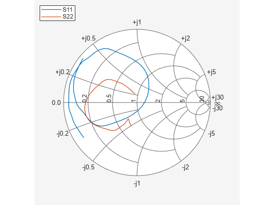
Plot Amplifier S11 and S22 Parameters
Use the smithplot method of circuit object to plot the original S11 and S22 parameters of the amplifier (SecondCkt) on a Z Smith® Chart. The original frequencies of the amplifier's S-parameters range from 1.0 GHz to 2.9 GHz.
fig = figure;
smithplot(SecondCkt,[1 1;2 2],Parent=fig);
Plot Amplifier Pin-Pout Data
Use the plot method of circuit object to plot the amplifier (SecondCkt) Pin-Pout data, in dBm, at 2.1 GHz on an X-Y plane.
figure
plot(SecondCkt,'Pout','dBm')
legend(Location="northwest");
![Figure contains an axes object. The axes object with xlabel P indexOf in baseline [dBm], ylabel dBm contains an object of type line. This object represents P_{out}(Freq=2.1[GHz]).](../../examples/rf/win64/RFCircuitObjectsExample_02.png)
Get Original Frequency Data and Result of Analyzing Amplifier over Original Frequencies
When the RF Toolbox reads data from default.amp into an amplifier object (SecondCkt), it also analyzes the amplifier over the frequencies of network parameters in default.amp file and store the result at the property AnalyzedResult. Here are the original amplifier frequency and analyzed result over it.
f = SecondCkt.AnalyzedResult.Freq;
data = SecondCkt.AnalyzedResult
data =
   rfdata.data with properties:

            Freq: [191×1 double]
    S_Parameters: [2×2×191 double]
      GroupDelay: [191×1 double]
              NF: [191×1 double]
            OIP3: [191×1 double]
              Z0: 50.0000 + 0.0000i
              ZS: 50.0000 + 0.0000i
              ZL: 50.0000 + 0.0000i
        IntpType: 'Cubic'
            Name: 'Data object'
Analyze and Plot S11 and S22 of Amplifier Circuit with Different Frequencies
To visualize the S-parameters of a circuit over a different frequency range, you must first analyze it over the specified frequency range.
analyze(SecondCkt,1.85e9:1e7:2.55e9);
fig = figure;
smithplot(SecondCkt,[1 1;2 2],GridType="ZY",Parent=fig)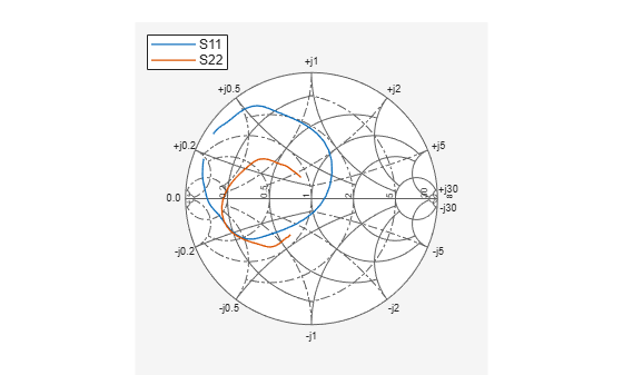
Create and Analyze Cascaded rfckt Object
Cascade three circuit objects to create a cascaded circuit object, and then analyze it at the original amplifier frequencies which range from 1.0 GHz to 2.9 GHz.
CascadedCkt = rfckt.cascade('Ckts',{FirstCkt,SecondCkt,ThirdCkt});
analyze(CascadedCkt,f)
ans =
rfckt.cascade with properties:
Ckts: {[1×1 rfckt.txline] [1×1 rfckt.amplifier] [1×1 rfckt.txline]}
nPort: 2
AnalyzedResult: [1×1 rfdata.data]
Name: 'Cascaded Network'
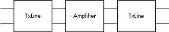
Figure 1: The cascaded circuit.
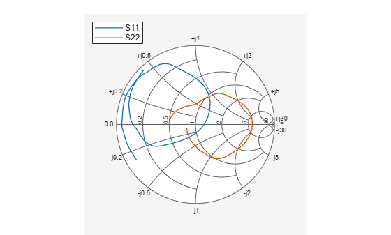
Plot S11 and S22 Parameters of Cascaded Circuit
Use the smithplot method of circuit object to plot S11 and S22 of the cascaded circuit (CascadedCkt) on a Z Smith chart.
fig = figure;
smithplot(CascadedCkt,[1 1;2 2],'GridType','Z','Parent',fig)
Plot S21 Parameters of Cascaded Circuit
Use the plot method of circuit object to plot S21 of the cascaded circuit (CascadedCkt) on an X-Y plane.
figure
plot(CascadedCkt,'S21','dB')
![Figure contains an axes object. The axes object with xlabel Freq [GHz], ylabel Magnitude (decibels) contains an object of type line. This object represents S_{21}.](../../examples/rf/win64/RFCircuitObjectsExample_06.png)
Plot Budget S21 Parameters and Noise Figure of Cascaded Circuit
Use the plot method of circuit object to plot the budget S21 parameters and noise figure of the cascaded circuit (CascadedCkt) on an X-Y plane.
figure
plot(CascadedCkt,'budget','S21','NF')
![Figure contains an axes object. The axes object with xlabel Freq [GHz], ylabel Stage of cascade contains 2 objects of type line. These objects represent S_{21}, NF.](../../examples/rf/win64/RFCircuitObjectsExample_07.png)