Credit Scoring Using Logistic Regression and Decision Trees
This example shows how to create and compare two credit scoring models, which includes:
Training both a logistic regression model (base model) and a decision tree model (challenger model) to predict PDs.
Validating the models by comparing the values of different validation metrics between the challenger model and the base model.
In this example, the base model is a logistic regression model, whereas the challenger model is a decision tree model. This example compares a credit scorecard logistic regression model (using creditscorecard) and decision tree scoring model (using fitctree), and presents a workflow to train the models, compute the PDs, and perform model validation using the risk.validation namespace. The models in this example are straightforward and trained using basic options for illustrative purposes, but you can use this workflow to compare more sophisticated champion and challenger models.
Compute Probabilities of Default Using Logistic Regression
First, create a scoring model using creditscorecard. Apply automatic binning using the autobinning function and use the default autobinning options. You can also use more advanced automatic and manual binning operations to improve the model by using the Binning Explorer. To train a logistic regression model, use fitmodel with the full model option to include all predictors in the model. Then, compute the PDs using probdefault. For a detailed description of this workflow, see Bin Data to Create Credit Scorecards Using Binning Explorer or Case Study for Credit Scorecard Analysis.
% Create a creditscorecard object, bin data, and fit a logistic regression model
load CreditCardData.mat
scl = creditscorecard(data,'IDVar','CustID');
scl = autobinning(scl);
scl = fitmodel(scl,'VariableSelection','fullmodel');
Generalized linear regression model:
    logit(status) ~ 1 + CustAge + TmAtAddress + ResStatus + EmpStatus + CustIncome + TmWBank + OtherCC + AMBalance + UtilRate
    Distribution = Binomial

Estimated Coefficients:
                   Estimate        SE         tStat        pValue
                   _________    ________    _________    __________

    (Intercept)      0.70246    0.064039       10.969    5.3719e-28
    CustAge           0.6057     0.24934       2.4292      0.015131
    TmAtAddress       1.0381     0.94042       1.1039       0.26963
    ResStatus         1.3794      0.6526       2.1137      0.034538
    EmpStatus        0.89648     0.29339       3.0556     0.0022458
    CustIncome       0.70179     0.21866       3.2095     0.0013295
    TmWBank           1.1132     0.23346       4.7683    1.8579e-06
    OtherCC           1.0598     0.53005       1.9994      0.045568
    AMBalance         1.0572     0.36601       2.8884     0.0038718
    UtilRate       -0.047597     0.61133    -0.077858       0.93794


1200 observations, 1190 error degrees of freedom
Dispersion: 1
Chi^2-statistic vs. constant model: 91, p-value = 1.05e-15
% Compute the corresponding probabilities of default
pdL = probdefault(scl);
Compute Probabilities of Default Using Decision Trees
Next, create the challenger model. Use the Statistics and Machine Learning Toolbox™ method fitctree to fit a Decision Tree (DT) to the data. By default, the splitting criterion is Gini's diversity index. In this example, set a maximum number of splits to avoid overfitting and specify which predictors are categorical. For information on additional training options that can improve the model, see the Name-Value Arguments in fitctree.
% Create and view classification tree
CategoricalPreds = {'ResStatus','EmpStatus','OtherCC'};
dt = fitctree(data,'status~CustAge+TmAtAddress+ResStatus+EmpStatus+CustIncome+TmWBank+OtherCC+UtilRate',...
    'MaxNumSplits',30,'CategoricalPredictors',CategoricalPreds);
disp(dt)
  ClassificationTree
           PredictorNames: {'CustAge'  'TmAtAddress'  'ResStatus'  'EmpStatus'  'CustIncome'  'TmWBank'  'OtherCC'  'UtilRate'}
             ResponseName: 'status'
    CategoricalPredictors: [3 4 7]
               ClassNames: [0 1]
           ScoreTransform: 'none'
          NumObservations: 1200


  Properties, Methods
The decision tree is shown below. You can also use the view function with the name-value argument mode set to "graph" to visualize the tree as a graph.
view(dt)
Decision tree for classification
 1  if CustIncome<30500 then node 2 elseif CustIncome>=30500 then node 3 else 0
 2  if TmWBank<60 then node 4 elseif TmWBank>=60 then node 5 else 1
 3  if TmWBank<32.5 then node 6 elseif TmWBank>=32.5 then node 7 else 0
 4  if TmAtAddress<13.5 then node 8 elseif TmAtAddress>=13.5 then node 9 else 1
 5  if UtilRate<0.255 then node 10 elseif UtilRate>=0.255 then node 11 else 0
 6  if CustAge<60.5 then node 12 elseif CustAge>=60.5 then node 13 else 0
 7  if CustAge<46.5 then node 14 elseif CustAge>=46.5 then node 15 else 0
 8  if CustIncome<24500 then node 16 elseif CustIncome>=24500 then node 17 else 1
 9  if TmWBank<56.5 then node 18 elseif TmWBank>=56.5 then node 19 else 1
10  if CustAge<21.5 then node 20 elseif CustAge>=21.5 then node 21 else 0
11  class = 1
12  if EmpStatus=Employed then node 22 elseif EmpStatus=Unknown then node 23 else 0
13  if TmAtAddress<131 then node 24 elseif TmAtAddress>=131 then node 25 else 0
14  if TmAtAddress<97.5 then node 26 elseif TmAtAddress>=97.5 then node 27 else 0
15  class = 0
16  class = 0
17  if ResStatus in {Home Owner Tenant} then node 28 elseif ResStatus=Other then node 29 else 1
18  if TmWBank<52.5 then node 30 elseif TmWBank>=52.5 then node 31 else 0
19  class = 1
20  class = 1
21  class = 0
22  if UtilRate<0.375 then node 32 elseif UtilRate>=0.375 then node 33 else 0
23  if UtilRate<0.005 then node 34 elseif UtilRate>=0.005 then node 35 else 0
24  if CustIncome<39500 then node 36 elseif CustIncome>=39500 then node 37 else 0
25  class = 1
26  if UtilRate<0.595 then node 38 elseif UtilRate>=0.595 then node 39 else 0
27  class = 1
28  class = 1
29  class = 0
30  class = 1
31  class = 0
32  class = 0
33  if UtilRate<0.635 then node 40 elseif UtilRate>=0.635 then node 41 else 0
34  if CustAge<49 then node 42 elseif CustAge>=49 then node 43 else 1
35  if CustIncome<57000 then node 44 elseif CustIncome>=57000 then node 45 else 0
36  class = 1
37  class = 0
38  class = 0
39  if CustIncome<34500 then node 46 elseif CustIncome>=34500 then node 47 else 1
40  class = 1
41  class = 0
42  class = 1
43  class = 0
44  class = 0
45  class = 1
46  class = 0
47  class = 1
The decision tree has a predict function, where the first output predicts the class and the second output provides the probability of belonging to that class.
% Extract probabilities of default
[~,ObservationClassProb] = predict(dt,data);
pdDT = ObservationClassProb(:,2);
ObservationClassProb returns a NumObs-by-2 array with class probability at all observations. The order of the classes is the same as in dt.ClassName. In this example, the class names are [0 1], where 0 represents the good label based on the class with the highest count in the raw data. The first column corresponds to nondefaults, whereas the second column represents the actual PDs. You use the PDs in the scoring or validation sections of the workflow.
Predictor Importance for Credit Scorecard Model
Predictor importance is related to the concept of predictor weights, as the weight of a predictor determines its significance in calculating the final score and the PD. For credit scorecards, the weights are determined by dividing the range of points for each predictor by the total range of points for the entire credit scorecard model.
In this example, use the formatpoints function with the PointsOddsandPDO name-value argument for scaling. Set the following parameters:
Target points
Target odds
Number of points to double the odds (PDO)
The odds double with every increase of points-to-double-the-odds (PDO). The formatpoints function solves for the scaling parameters so that the scaled scores are consistent with the target points, the target odds, and the PDO.
% Choose target points, target odds, and PDO values
TargetPoints = 500;
TargetOdds = 2;
PDO = 50;

% Format points and compute points range
scl = formatpoints(scl,'PointsOddsAndPDO',[TargetPoints TargetOdds PDO]);
[PointsTable,MinPts,MaxPts] = displaypoints(scl);
PtsRange = MaxPts - MinPts;
disp(PointsTable(1:10,:))
      Predictors            Bin         Points
    _______________    _____________    ______

    {'CustAge'    }    {'[-Inf,33)'}    37.008
    {'CustAge'    }    {'[33,37)'  }    38.342
    {'CustAge'    }    {'[37,40)'  }    44.091
    {'CustAge'    }    {'[40,46)'  }    51.757
    {'CustAge'    }    {'[46,48)'  }    63.826
    {'CustAge'    }    {'[48,58)'  }     64.97
    {'CustAge'    }    {'[58,Inf]' }    82.826
    {'CustAge'    }    {'<missing>'}       NaN
    {'TmAtAddress'}    {'[-Inf,23)'}    49.058
    {'TmAtAddress'}    {'[23,83)'  }    57.325
fprintf('Minimum points: %g, Maximum points: %g\n',MinPts,MaxPts)Minimum points: 348.705, Maximum points: 683.668
The weights are defined as the range of points, for any given predictor, divided by the range of points for the entire scorecard.
Predictor = unique(PointsTable.Predictors,'stable');
NumPred = length(Predictor);
Weight  = zeros(NumPred,1);

for ii = 1 : NumPred
   Ind = strcmpi(Predictor{ii},PointsTable.Predictors);
   MaxPtsPred = max(PointsTable.Points(Ind));
   MinPtsPred = min(PointsTable.Points(Ind));
   Weight(ii) = 100*(MaxPtsPred-MinPtsPred)/PtsRange;
end

PredictorWeights = table(Predictor,Weight);
PredictorWeights(end+1,:) = PredictorWeights(end,:);
PredictorWeights.Predictor{end} = 'Total';
PredictorWeights.Weight(end) = sum(Weight);
disp(PredictorWeights)
       Predictor       Weight
    _______________    _______

    {'CustAge'    }     13.679
    {'TmAtAddress'}     5.1564
    {'ResStatus'  }     8.7945
    {'EmpStatus'  }      8.519
    {'CustIncome' }     19.259
    {'TmWBank'    }     24.557
    {'OtherCC'    }     7.3414
    {'AMBalance'  }     12.365
    {'UtilRate'   }    0.32919
    {'Total'      }        100
% Plot a histogram of the weights
figure
bar(PredictorWeights.Weight(1:end-1))
title('Predictor Importance Estimates for Credit Scorecard');
ylabel('Estimates (%)');
xlabel('Predictors');
xticklabels(PredictorWeights.Predictor(1:end-1));

Using Decision Trees for Predictor Importance
When you use decision trees, you can investigate predictor importance using the predictorImportance function. On every predictor, the function sums and normalizes changes in the risks due to splits by using the number of branch nodes. A high value in the output array indicates a strong predictor.
imp = predictorImportance(dt);

figure;
bar(100*imp/sum(imp)); % to normalize on a 0-100% scale
title('Predictor Importance Estimates for Decision Tree');
ylabel('Estimates (%)');
xlabel('Predictors');
xticklabels(dt.PredictorNames);

In this case, 'CustIncome' (parent node) is the most important predictor, followed by 'UtilRate', where the second split happens, and so on. The predictor importance step can help in predictor screening for data sets with a large number of predictors.
Normalize the predictor importance for decision trees using a percent from 0 through 100%, then compare the two models in a combined histogram.
Ind = ismember(Predictor,dt.PredictorNames);
w = zeros(size(Weight));
w(Ind) = 100*imp'/sum(imp);
figure
bar([Weight,w]);
title('Predictor Importance Estimates');
ylabel('Estimates (%)');
xlabel('Predictors');
h = gca;
xticklabels(Predictor)
legend({'logit','DT'})

Comparing the predictor importance of the two models, not only are the weights across models different, but the selected predictors in each model also diverge. The predictors 'AMBalance' and 'OtherCC' are missing from the decision tree model, and 'UtilRate' is missing from the logistic regression model.
Note that these results depend on the binning algorithm you choose for the creditscorecard object and the parameters used in fitctree to build the decision tree. Different parameter choices made during training may bring the importance of different predictors closer across models.
Model Validation
You can use various validation tools from the toolbox to access and compare these models. For instance, both creditscorecard and decision trees offer validation tools. crediscorecard supports a validatemodel function that supports discrimination metrics and visualizations. Decision trees have tools such as the predictorImportance function used earlier, tools for cross validation (Improving Classification Trees and Regression Trees), and tools for interpretability (Interpret Machine Learning Models). However, not all validation tools supported in the scorecard are supported by decision trees, and vice versa. The risk.validation namespace offers a convenient way to compute the same validation metrics for any model and compare the results.
This example performs in-sample validation, where you use the same data set for both training and validating the models. Alternatively, you can split the data into training and testing, retrain the models with the training set, and use the test data to perform out-of-sample validation.
Recall the PD from the scorecard is stored in the variable pdL, and the decision tree PD is stored in pdDT. For validation, you need the predicted PDs and the binary response. In this case, the response data is in data.status. In this section, you arrange the validation data (predictions by both models and response values) in a new table.
ValidationData = table(pdL,pdDT,data.status,VariableNames=["PDScorecard" "PDDecisionTree" "DefaultFlag"]);
head(ValidationData)
    PDScorecard    PDDecisionTree    DefaultFlag
    ___________    ______________    ___________

      0.24717          0.19672            0
      0.20283         0.090909            0
      0.31063          0.19672            0
       0.1677          0.26977            0
      0.18661         0.090909            0
      0.14176          0.19672            0
      0.51817          0.40323            1
       0.2793          0.19672            0
Once you have trained and validated your models, you can use discrimination metrics to measure how well models can differentiate between different outcomes. The next section highlights a set of discrimination metrics you can use in your workflows.
Discrimination
Discrimination measures how well the model predictions rank the customers by risk. Higher risk customers should be assigned riskier scores such as higher PD values. In this section, compute the following discrimination metrics:
Accuracy ratio (AR) –
risk.validation.accuracyRatioArea under the curve (AUC) –
risk.validation.areaUnderCurveKolmogorov-Smirnov (KS) –
risk.validation.kolmogorovSmirnovBrier score –
risk.validation.brierScore
This example includes Brier score as a discrimination metric, although it can also be used as a calibration metric in other applications.
DiscriminationResults = table;
DiscriminationResults.AR = zeros(2,1); % Accuracy ratio
DiscriminationResults.AUC = zeros(2,1); % Area under the curve
DiscriminationResults.KS = zeros(2,1); % Kolmogorov-Smirnov
DiscriminationResults.Brier = zeros(2,1); % Brier score
DiscriminationResults.Properties.RowNames = ["Scorecard"; "Decision Tree"];

for ii=1:2 % for each model
   PDVar = ValidationData.Properties.VariableNames{ii};
   DiscriminationResults.AR(ii) = risk.validation.accuracyRatio(ValidationData.(PDVar),ValidationData.DefaultFlag);
   DiscriminationResults.AUC(ii) = risk.validation.areaUnderCurve(ValidationData.(PDVar),ValidationData.DefaultFlag);
   DiscriminationResults.KS(ii) = risk.validation.kolmogorovSmirnov(ValidationData.(PDVar),ValidationData.DefaultFlag);
   DiscriminationResults.Brier(ii) = risk.validation.brierScore(ValidationData.(PDVar),ValidationData.DefaultFlag);
end
disp(DiscriminationResults)
                       AR         AUC        KS        Brier
                     _______    _______    _______    _______

    Scorecard        0.32515    0.66258    0.23204    0.20519
    Decision Tree    0.38903    0.69451    0.29666    0.19166
For AR, AUC and KS, higher values mean better discrimination, whereas for Brier score, lower values indicate better discrimination. These are simple models, included here for illustration purposes, and there should be no general conclusions about these classes of models based on these results. Both models can be improved with additional tuning during training.
A deciles report is commonly used when analyzing model discrimination. This report groups the portfolio data into deciles by PD, and then displays a range of metrics for each decile.
Select a model using the dropdown to generate the deciles report for the corresponding model. The risk.validation.thresholdMetrics function generates the information needed for the report.
Model ="Scorecard"; if Model=="Scorecard" PDVar = "PDScorecard"; else PDVar = "PDDecisionTree"; end PDSelected = ValidationData.(PDVar); DecileNumberByPD = risk.validation.groupNumberByQuantile(PDSelected,"deciles"); PDAvgByDecile = groupsummary(PDSelected,DecileNumberByPD,"mean"); PDMappedToDecilePD = PDAvgByDecile(DecileNumberByPD); metricsByDecile = risk.validation.thresholdMetrics(PDMappedToDecilePD,ValidationData.DefaultFlag); disp(metricsByDecile)
    Threshold    TruePositiveRate    FalsePositiveRate    RateOfPositivePredictions    TruePositives    FalsePositives    TrueNegatives    FalseNegatives
    _________    ________________    _________________    _________________________    _____________    ______________    _____________    ______________

     0.58115               0                    0                      0                      0                0               803              397
     0.58115         0.17632             0.062267                    0.1                     70               50               753              327
     0.46854         0.32242              0.13948                    0.2                    128              112               691              269
     0.41592         0.44081              0.23039                    0.3                    175              185               618              222
      0.3696          0.5466              0.32752                    0.4                    217              263               540              180
     0.33316         0.64736              0.42715                    0.5                    257              343               460              140
     0.29963         0.74055              0.53051                    0.6                    294              426               377              103
     0.27108         0.82872              0.63636                    0.7                    329              511               292               68
     0.23646         0.90176              0.74969                    0.8                    358              602               201               39
     0.19635         0.96725              0.86675                    0.9                    384              696               107               13
     0.13643               1                    1                      1                    397              803                 0                0
Reformat the table to reflect the meaning of these metrics in the context of credit risk. "Bads" in the column names refers to defaulters, whereas "Goods" refers to nondefaulters.
decileReport = renamevars(metricsByDecile,metricsByDecile.Properties.VariableNames,...
   ["PD" "Proportion of Bads" "Proportion of Goods" "Proportion of Borrowers" "Cumulative Bads" "Cumulative Goods" "Goods in Higher Deciles" "Bads in Higher Deciles"]);
decileReport(1,:) = []; % First row is mostly for plotting purposes
decileReport = addvars(decileReport,(1:height(decileReport))',Before="PD",NewVariableNames="Decile");
disp(decileReport)
    Decile      PD       Proportion of Bads    Proportion of Goods    Proportion of Borrowers    Cumulative Bads    Cumulative Goods    Goods in Higher Deciles    Bads in Higher Deciles
    ______    _______    __________________    ___________________    _______________________    _______________    ________________    _______________________    ______________________

       1      0.58115         0.17632               0.062267                    0.1                     70                 50                     753                       327
       2      0.46854         0.32242                0.13948                    0.2                    128                112                     691                       269
       3      0.41592         0.44081                0.23039                    0.3                    175                185                     618                       222
       4       0.3696          0.5466                0.32752                    0.4                    217                263                     540                       180
       5      0.33316         0.64736                0.42715                    0.5                    257                343                     460                       140
       6      0.29963         0.74055                0.53051                    0.6                    294                426                     377                       103
       7      0.27108         0.82872                0.63636                    0.7                    329                511                     292                        68
       8      0.23646         0.90176                0.74969                    0.8                    358                602                     201                        39
       9      0.19635         0.96725                0.86675                    0.9                    384                696                     107                        13
      10      0.13643               1                      1                      1                    397                803                       0                         0
The Proportion of Borrowers column shows the proportion of the entire portfolio that is included up to that row in the table. For the scorecard model, this has increments of 0.1, as expected, since these are the deciles. The Proportion of Bads and Proportion of Goods columns show that for the 10% of the portfolio with the highest PD, about 17.6% of the defaulters have been identified, and only about 6.2% of the nondefaulters where assigned such high PD value. For 20% of the portfolio, the model already correctly labeled 32.2% of the defaulters, and only incorrectly labeled 13.9% of the nondefaulters as risky. An ideal model would show the Proportion of Bads increasing quickly while the Proportion of Goods stays low initially and only grows towards the bottom of the table where PD values are low and Cumulative Goods are high.
For the decision tree model in this example, there are only 6 rows and the proportion in each row does not match 10%. This is because the model tends to predict some PD values very often. Here is the frequency table of the predicted PD values for the decision tree model.
tabulate(ValidationData.PDDecisionTree)
      Value    Count   Percent
     0.0625       16      1.33%
  0.0909091       44      3.67%
   0.166667        6      0.50%
   0.196721      244     20.33%
        0.2        5      0.42%
       0.25       20      1.67%
   0.252688      186     15.50%
   0.269767      215     17.92%
   0.285714        7      0.58%
   0.333333        3      0.25%
   0.403226      248     20.67%
        0.5        8      0.67%
   0.513761      109      9.08%
   0.571429        7      0.58%
   0.645161       31      2.58%
   0.666667        9      0.75%
   0.727273       11      0.92%
          1       31      2.58%
The tabulated output shows the various percentages of the portfolio and the associated PD. For example, the first row indicates that 1.33% of the portfolio gets a PD of 6.25%. It is not possible to split the portfolio into bins with exactly 10% of observations when using the PD value as the split criterion. In this case, when determining the deciles, the data ends up grouped into 6 bins, where some bins contain over 20% of observations.
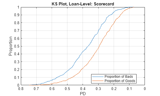
The Kolmogorov-Smirnov plot precisely shows the growth of the proportion of bads and the proportion of goods for a model, as a function of the PD value (or a score value). Typically, it is sorted from riskier scores on the left (such as high PD) to safer scores on the right (such as low PD). The KS metric is the maximum difference between these proportions.
figure;
plot(metricsByDecile.Threshold,metricsByDecile.TruePositiveRate)
hold on
plot(metricsByDecile.Threshold,metricsByDecile.FalsePositiveRate)
hold off
grid on
ax = gca;
ax.XDir = "reverse";
title(strcat("KS Plot by Deciles: ",Model))
xlabel("PD")
ylabel("Proportion")
legend("Proportion of Bads","Proportion of Goods",Location="best")

The receiver operating characteristic (ROC) curve plots the Proportion of Bads versus the Proportion of Goods directly, without showing the PD values.
figure;
plot(flipud(metricsByDecile.FalsePositiveRate),flipud(metricsByDecile.TruePositiveRate))
grid on
title(strcat("ROC by Deciles: ",Model))
xlabel("Proportion of Goods")
ylabel("Proportion of Bads")
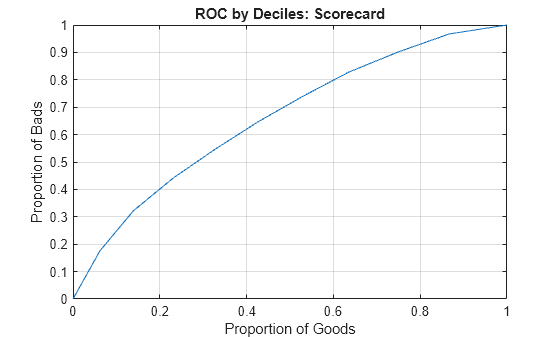
In this case, a curve that quickly increases is preferred, since this shows that the defaulters are identified faster than the nondefaulters, while the score or PD changes from riskier to safer values.
You can generate either plot at the individual loan level as well, without aggregating by deciles. For example, you can make the KS plot at the loan level by using the following code.
[ksValue,ksOutput] = risk.validation.kolmogorovSmirnov(ValidationData.(PDVar),ValidationData.DefaultFlag);
figure;
plot(ksOutput.Metrics.Threshold,ksOutput.Metrics.TruePositiveRate)
hold on
plot(ksOutput.Metrics.Threshold,ksOutput.Metrics.FalsePositiveRate)
hold off
grid on
ax = gca;
ax.XDir = "reverse";
title(strcat("KS Plot, Loan-Level: ",Model))
xlabel("PD")
ylabel("Proportion")
legend("Proportion of Bads","Proportion of Goods",Location="best")
Calibration
Model calibration measures how close the predicted PDs are from the actual default rates. It requires grouping individual loans so that a default rate for the group can be computed and compared to the average PD of the group. For individual loans, the response value is a 0 or 1 value, whereas the predicted PD for the loan is a continuous value. By grouping, you can measure the default rate within a group (the number of defaults divided by the number of loans), which is a value between 0 and 1, and compare it to the group's PD.
For credit scoring models, where each individual borrower may get its own PD value, it is common to use deciles as groups. For credit rating models, each rating is a natural group.
Some calibration metrics, such as the Hosmer-Lemeshow test and the root mean square error (RMSE), require all the groups in the portfolio to compute a single calibration value for the portfolio.
Hosmer-Lemeshow is a statistical test where the null hypothesis states that the expected number of defaults in the groups matches the observed defaults. A rejection of the null hypothesis means that expected and observed default counts are not close enough and the models should be reviewed. In this example, we report the rejection flag and the corresponding p-value (smaller values suggest mismatch between expected and observed defaults). For more information about this test, see risk.validation.hosmerLemeshowTest.
The RMSE metric rmse is the average value of the square errors between the predicted PD and observed default rate.
CalibrationResults = table;
CalibrationResults.HosmerLemeshowReject = zeros(2,1); % Hosmer-Lemeshow test rejection flag
CalibrationResults.HosmerLemeshowPValue = zeros(2,1); % Hosmer-Lemeshow test p-value
CalibrationResults.RMSE = zeros(2,1); % Root mean square error
CalibrationResults.Properties.RowNames = ["Scorecard"; "Decision Tree"];

for ii=1:2 % for each model
   PDVar = ValidationData.Properties.VariableNames{ii};
   PDSelected = ValidationData.(PDVar);

   DecileNumberByPD = risk.validation.groupNumberByQuantile(PDSelected,"deciles");
   PDAvgByDecile = groupsummary(PDSelected,DecileNumberByPD,"mean");
   [NumDefaultsByDecile,~,NumLoansByDecile] = groupsummary(ValidationData.DefaultFlag,DecileNumberByPD,"sum");

   [HLReject,HLOutput] = risk.validation.hosmerLemeshowTest(PDAvgByDecile,NumDefaultsByDecile,NumLoansByDecile);
   CalibrationResults.HosmerLemeshowReject(ii) = HLReject;
   CalibrationResults.HosmerLemeshowPValue(ii) = HLOutput.PValue;
   CalibrationResults.RMSE(ii) = rmse(PDAvgByDecile,NumDefaultsByDecile./NumLoansByDecile,Weight=NumLoansByDecile);
end
disp(CalibrationResults)
                     HosmerLemeshowReject    HosmerLemeshowPValue       RMSE
                     ____________________    ____________________    __________

    Scorecard                 0                    0.97998             0.017103
    Decision Tree             0                          1           9.2096e-16
You can interpret the following results from the table:
The rejection flag is
0signifying a good fit between expected and observed defaults.A higher p-value indicates better performance.
A lower RMSE indicates better performance.
Other calibration tests such as the binomial test, measure the calibration for each individual group. For more information about this test, see risk.validation.binomialTest. For the binomial test, the null hypothesis states that the PD for each group matches the group's default rate. Rejection of the test means that the PD underestimates the default rate. As before, deciles are commonly used for grouping.
Model ="Scorecard"; if Model=="Scorecard" PDVar = "PDScorecard"; else PDVar = "PDDecisionTree"; end PDSelected = ValidationData.(PDVar); DecileNumberByPD = risk.validation.groupNumberByQuantile(PDSelected,"deciles"); PDAvgByDecile = groupsummary(PDSelected,DecileNumberByPD,"mean"); [NumDefaultsByDecile,~,NumLoansByDecile] = groupsummary(ValidationData.DefaultFlag,DecileNumberByPD,"sum"); [BinTestReject,BinTestOutput] = risk.validation.binomialTest(PDAvgByDecile,NumDefaultsByDecile,NumLoansByDecile);
You can see that each group has its own test result. The main output of the function shows the rejection flag for each group.
disp(BinTestReject)
     0
     0
     0
     0
     0
     0
     0
     0
     0
     0
The structure BinTestOutput contains a table with detailed information about the test results for each group. The first column of the table displays the rejection flag for the test.
disp(BinTestOutput.Results)
    RejectBinTest    PValue     NumEvents    CriticalValue    ConfidenceLevel    NumTrials    Probability    ObservedProbability
    _____________    _______    _________    _____________    _______________    _________    ___________    ___________________

          0           0.8493       13             24               0.95             120         0.13643            0.10833
          0          0.32138       26             32               0.95             120         0.19635            0.21667
          0          0.48175       29             37               0.95             120         0.23646            0.24167
          0          0.33819       35             42               0.95             120         0.27108            0.29167
          0           0.4516       37             45               0.95             120         0.29963            0.30833
          0           0.5327       40             50               0.95             120         0.33316            0.33333
          0           0.7031       42             54               0.95             120          0.3696               0.35
          0          0.73511       47             60               0.95             120         0.41592            0.39167
          0          0.40712       58             66               0.95             120         0.46854            0.48333
          0          0.51955       70             80               0.95             120         0.58115            0.58333
The binomial test assumes the defaults are independent. To assess the effect of correlation between events, you can apply the correlated binomial test, which requires a correlation value as an additional input parameter. This example uses a 10% correlation for illustration purposes. For more information about the correlated binomial test, see risk.validation.correlatedBinomialTest.
CorrValue = 0.1;
[~,CorrBinTestOutput] = risk.validation.correlatedBinomialTest(PDAvgByDecile,NumDefaultsByDecile,NumLoansByDecile,CorrValue);
disp(CorrBinTestOutput.Results)
    RejectCorrBinTest    PValue     NumEvents    CriticalValue    ConfidenceLevel    NumTrials    Probability    ObservedProbability    Correlation    EventCorrelation
    _________________    _______    _________    _____________    _______________    _________    ___________    ___________________    ___________    ________________

            0            0.60583       13             35               0.95             120         0.13643            0.10833              0.1            0.043043
            0            0.38439       26             46               0.95             120         0.19635            0.21667              0.1            0.050366
            0             0.4511       29             53               0.95             120         0.23646            0.24167              0.1            0.054047
            0             0.4075       35             58               0.95             120         0.27108            0.29167              0.1            0.056624
            0            0.45226       37             62               0.95             120         0.29963            0.30833              0.1            0.058393
            0            0.48512       40             67               0.95             120         0.33316            0.33333              0.1            0.060106
            0            0.55054       42             72               0.95             120          0.3696               0.35              0.1            0.061564
            0            0.56914       47             78               0.95             120         0.41592            0.39167              0.1            0.062864
            0            0.46487       58             84               0.95             120         0.46854            0.48333              0.1            0.063643
            0            0.51871       70             96               0.95             120         0.58115            0.58333              0.1            0.062926
The critical values are higher for the correlated binomial test, showing that a higher number of defaults is acceptable under the assumption that there is some level of correlation between defaults.
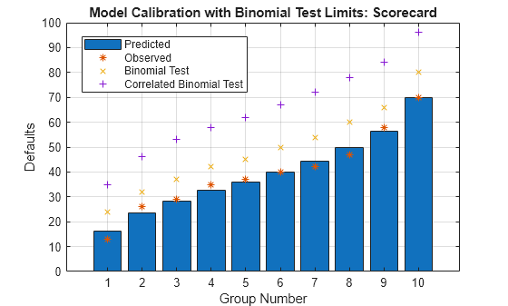
The following plot summarizes the calibration results from the uncorrelated and correlated binomial tests.
figure;
bar(BinTestOutput.Results.Probability.*BinTestOutput.Results.NumTrials)
hold on
plot(BinTestOutput.Results.NumEvents,'*')
plot(BinTestOutput.Results.CriticalValue,'x')
plot(CorrBinTestOutput.Results.CriticalValue,'+')
hold off
grid on
legend("Predicted","Observed","Binomial Test","Correlated Binomial Test",Location="best")
xlabel("Group Number")
ylabel("Defaults")
title(strcat("Model Calibration with Binomial Test Limits: ",Model))
You can improve the simple models that this example compares with additional parameter tuning during training. This example also demonstrates readily available tools that you can use to train and validate credit scoring models.
More About
Logistic regression links the score and the PD through the logistic regression function, and is the default fitting and scoring model when you work with creditscorecard objects. Decision trees have gained popularity in credit scoring and are now commonly used to fit data and predict default. The decision trees algorithms follow a top-down approach where the data set is split according to a chosen metric, including the Gini index, information value, or entropy. For more information, see Decision Trees. The Risk Model Validation offers a range of tools to validate and compare the models.
See Also
creditscorecard | autobinning | fitmodel | displaypoints | formatpoints | probdefault | validatemodel
Topics
- Feature Screening with screenpredictors
- Credit Rating by Bagging Decision Trees
- Stress Testing of Consumer Credit Default Probabilities Using Panel Data
- About Credit Scorecards
- Credit Scorecard Modeling Workflow