Main Content

Transform Trajectory

Generate trajectory between two homogeneous transforms

  • Transform Trajectory block

Libraries:
Robotics System Toolbox / Utilities

Description

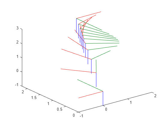
The Transform Trajectory block generates an interpolated trajectory between two homogenous transformation matrices. The block outputs the transform at the times given by the Time input, which can be a scalar or vector.

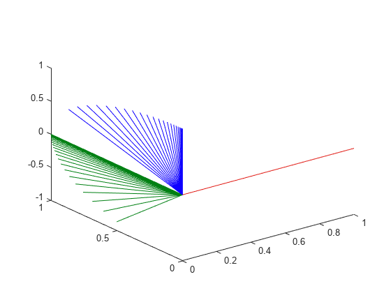
The trajectory is computed using quaternion spherical linear interpolation (SLERP) for the rotation and linear interpolation for the translation. This method finds the shortest path between positions and rotations of the transformation. Select the Use custom time scaling check box to compute the trajectory using a custom time scaling. The block uses linear time scaling by default.

The initial and final values are held constant outside the time period defined in Time interval.

Examples

Ports

Input

expand all

Time point along trajectory, specified as a scalar or vector. In general, when specified as a scalar, this value is synced with simulation time and is used to specify the time point for sampling the trajectory. The block outputs a vector of the trajectory variables at that instant in time. If the time is specified as a vector, the block outputs a matrix with each column corresponding to each element of the vector.

Data Types: single | double

Initial transformation matrix, specified as a 4-by-4 homogeneous transformation. The function generates a trajectory that starts at the initial orientation, T0, and goes to the final orientation, TF.

Example: trvec2tform([1 10 -1])

Dependencies

To enable this parameter, set the Waypoint source to External.

Data Types: single | double

Final transformation matrix, specified as a 4-by-4 homogeneous transformation. The function generates a trajectory that starts at the initial orientation, T0, and goes to the final orientation, TF.

Example: trvec2tform([1 10 -1])

Dependencies

To enable this parameter, set the Waypoint source to External.

Data Types: single | double

Start and end times for the trajectory, specified as a two-element vector.

Example: [0 10]

Dependencies

To enable this parameter, set the Waypoint source to External.

Data Types: single | double

Time scaling time points, specified as a scalar or n p-element vector, where p is the number of points for time scaling. By default, the time scaling is a linear time scaling spanning the TimeInterval. Specify the actual time scaling values in TimeScaling.

If the Time input is specified at a time not specified by these points, interpolation is used to find the right scaling time.

Dependencies

To enable this parameter, select the Use custom time scaling check box and set Parameter source to External.

To specify a scalar, the Time input must be a scalar.

Data Types: single | double

Time scaling vector and its first two derivatives, specified as a three element vector or a 3-by-p matrix, where m is the length of TSTime. By default, the time scaling is a linear time scaling spanning the TimeInterval.

For a nonlinear time scaling, specify the values of the time points in the first row. The second and third rows are the velocity and acceleration of the time points, respectively. For example, to follow the path with a linear velocity to the halfway point, and then jump to the end, the time-scaling would be:

s(1,:) = [0 0.25 0.5 1 1 1] % Position
s(2,:) = [1    1   1 0 0 0] % Velocity
s(3,:) = [0    0   0 0 0 0] % Acceleration

Dependencies

To enable this parameter, select the Use custom time scaling check box and set Parameter source to External.

To specify a three-element vector, the Time and TSTime inputs must be a scalar.

Data Types: single | double

Output

expand all

Homogeneous transformation matrices, returned as a 4-by-4-by-m homogenous matrix array, where m is the number of points input to Time.

Transform velocities, returned as a 6-by-m matrix, where m is the number of points input to Time. Each row of the vector is the angular and linear velocity of the transform as [wx wy wz vx vy vz]. w represents an angular velocity and v represents a linear velocity.

Transform velocities, returned as a 6-by-m matrix, where m is the number of points input to Time. Each row of the vector is the angular and linear acceleration of the transform as [alphax alphay alphaz ax ay az]. alpha represents an angular acceleration and a represents a linear acceleration.

Parameters

expand all

Specify External to specify the Waypoints and Time points parameters as block inputs instead of block parameters.

Initial transformation matrix, specified as a 4-by-4 homogeneous transformation. The function generates a trajectory that starts at the Initial transform and goes to the Final transform.

Data Types: single | double

Final transformation matrix, specified as a 4-by-4 homogeneous transformation. The function generates a trajectory that starts at the Initial transform and goes to the Final transform.

Data Types: single | double

Start and end times for the trajectory, specified as a two-element vector in seconds.

Data Types: single | double

Enable to specify custom time scaling for the trajectory using the Parameter Source, Time scaling time, and Time scaling values parameters.

Specify External to specify the Time scaling time and Time scaling values parameters as block inputs instead of block parameters.

Dependencies

To enable this parameter, select the Use custom time scaling check box.

Time scaling time points, specified as a scalar or p-element vector, where p is the number of points for time scaling. By default, the time scaling is a linear time scaling spanning the Time interval. Specify the actual time scaling values in Time scaling values.

If the Time input is specified at a time not specified by these points, interpolation is used to find the right scaling time.

Dependencies

To enable this parameter, select the Use custom time scaling check box.

To specify a scalar, the Time input must be a scalar.

Data Types: single | double

Time scaling vector and its first two derivatives, specified as a three-element vector or 3-by-p matrix, where p is the length of Time scaling time. By default, the time scaling is a linear time scaling spanning the Time interval.

For a nonlinear time scaling, specify the values of the time points in the first row. The second and third rows are the velocity and acceleration of the time points, respectively. For example, to follow the path with a linear velocity to the halfway point, and then jump to the end, the time-scaling would be:

s(1,:) = [0 0.25 0.5 1 1 1] % Position
s(2,:) = [1    1   1 0 0 0] % Velocity
s(3,:) = [0    0   0 0 0 0] % Acceleration

Dependencies

To enable this parameter, select the Use custom time scaling check box.

To specify a three-element vector, the Time and TSTime inputs must be a scalar.

Data Types: single | double

  • Interpreted execution — Simulate model using the MATLAB® interpreter. This option shortens startup time but has a slower simulation speed than Code generation. In this mode, you can debug the source code of the block.

  • Code generation — Simulate model using generated C code. The first time you run a simulation, Simulink generates C code for the block. The C code is reused for subsequent simulations, as long as the model does not change. This option requires additional startup time, but the speed of the subsequent simulations is comparable to Interpreted execution.

Tunable: No

Tips

For better performance, consider these options:

  • Minimize the number of waypoint or parameter changes.

  • Set the Waypoint source parameter to Internal.

  • Set the Simulate using parameter to Code generation. For more information, see Interpreted Execution vs. Code Generation (Simulink).

References

[1] Lynch, Kevin M., and Frank C. Park. Modern Robotics: Mechanics, Planning, and Control. Cambridge University Press, 2017.

Extended Capabilities

C/C++ Code Generation
Generate C and C++ code using Simulink® Coder™.

Version History

Introduced in R2019a
Go to top of page