A* Path Planning and Obstacle Avoidance in a Warehouse
This example is an extension to the Simulate a Mobile Robot in a Warehouse Using Gazebo example. The example shows to change the PRM path planner with an A* planner, and add a vector field histogram (VFH) algorithm to avoid obstacles.
Prerequisites
Review the Simulate a Mobile Robot in a Warehouse Using Gazebo example to setup the sensing and actuation elements. This example goes over how to download and use a virtual machine (VM) to setup a simulated robot.
Review the Execute Tasks for a Warehouse Robot example for the workflow of path planning and navigating in a warehouse scenario.
Model Overview
There are two major changes to this model from the Execute Tasks for a Warehouse Robot example. The goal is to replace the path planner algorithm used and add a controller that avoids obstacles in the environment.
The Planner MATLAB® Function Block now uses the plannerAStarGrid (Navigation Toolbox) object to run the A* path planning algorithm.
The Obstacle Avoidance subsystem now uses a Vector Field Histogram block as part of the controller. The rangeReadings function block outputs the ranges and angles when the data received is not empty. The VFH block then generates a steering direction based on obstacles within the scan range. For close obstacles, the robot should turn to drive around them. Tune the VFH parameters for different obstacle avoidance performance.
open_system("aStarPathPlanningAndObstacleAvoidanceInWarehouse.slx"); 
Setup
Warehouse Facility
Load the example map file, map, which is a matrix of logical values indicating occupied space in the warehouse. Invert this matrix to indicate free space, and create a binaryOccupancyMap object. Specify a resolution of 100 cells per meter.
The map is based off of the obstacleAvoidanceWorld.world, which is loaded in the VM. A PNG-file was generated to use as the map matrix with the collision_map_creator_plugin plugin. For more information, see Collision Map Creator Plugin.
close
figure("Name","Warehouse Map","Visible","on")
load exampleHelperWarehouseRobotWithGazeboBuses.mat
load helperPlanningAndObstacleAvoidanceWarehouseMap.mat map
logicalMap = map.getOccupancy;
mapScalingFactor = 100;
show(map)
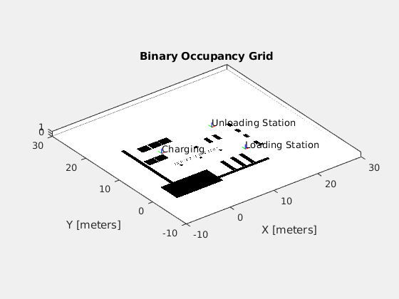
Assign the xy-locations of the charging station, sorting station, and the unloading location near shelves in the warehouse. The values chosen are based on the simulated world in Gazebo.
chargingStn = [2, 13];
loadingStn = [15, 5];
unloadingStn = [15, 15];
Show the various locations on the map.
hold on;
localOrigin = map.LocalOriginInWorld;
localTform = trvec2tform([localOrigin 0]);
text(chargingStn(1), chargingStn(2),1,'Charging');
plotTransforms([chargingStn, 0],[1 0 0 0])

text(loadingStn(1), loadingStn(2),1,'Loading Station');
plotTransforms([loadingStn, 0], [1 0 0 0])

text(unloadingStn(1), unloadingStn(2),1,'Unloading Station');
plotTransforms([unloadingStn, 0], [1 0 0 0])

hold off;
Simulate
To simulate the scenario, set up the connection to Gazebo.
First, run the Gazebo Simulator. In the virtual machine, click the Gazebo Warehouse Robot with Obstacles icon. If the Gazebo simulator fails to open, you may need to reinstall the plugin. See Install Gazebo Plugin Manually in Perform Co-Simulation Between Simulink and Gazebo.
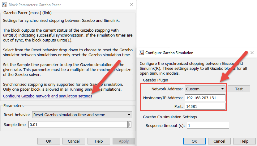
In Simulink, open the Gazebo Pacer block and click Configure Gazebo network and simulation settings. Specify the Network Address as Custom, the Hostname/IP Address for your Gazebo simulation, and a Port of 14581, which is the default port for Gazebo. The desktop of the VM displays the IP address.
For more information about connecting to Gazebo to enable co-simulation, see Perform Co-Simulation Between Simulink and Gazebo.
Click the Initialize Model button at the top of the model to initialize all the variables declared above.
Run the simulation. The robot drives around the environment and avoids unexpected obstacles.
sim("aStarPathPlanningAndObstacleAvoidanceInWarehouse.slx");
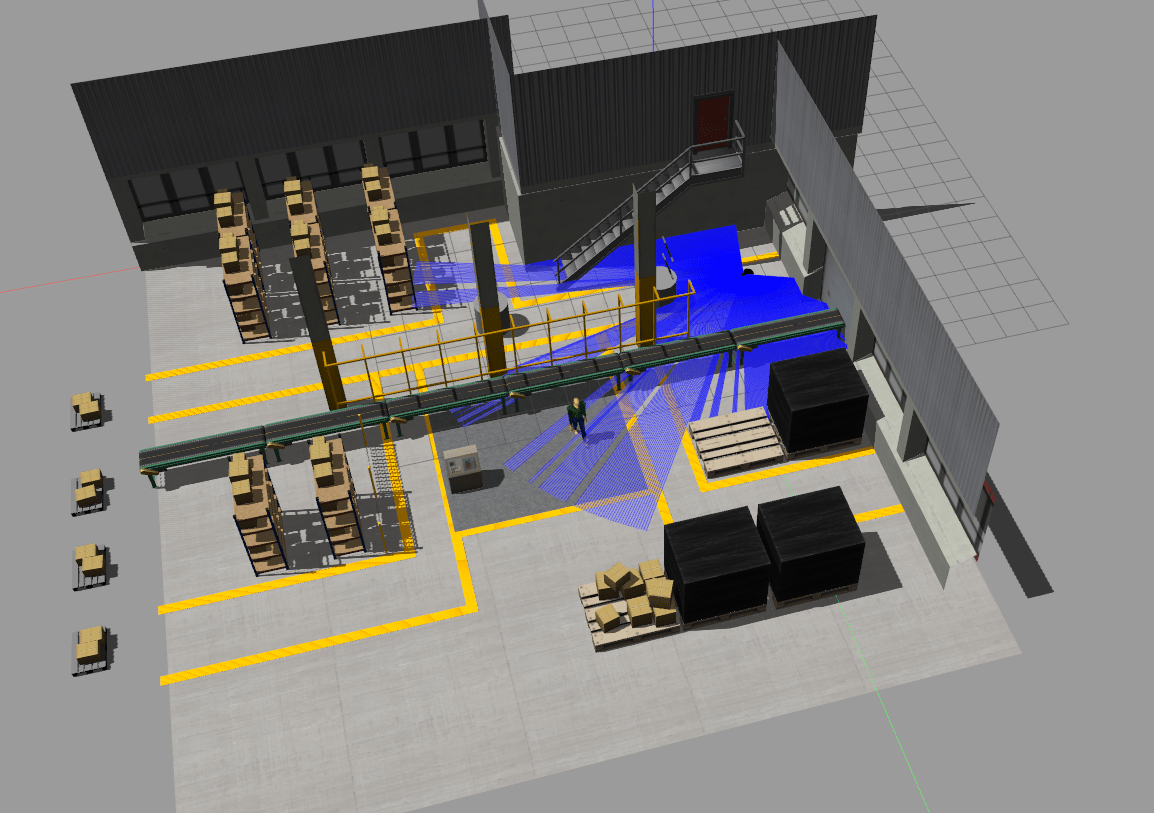
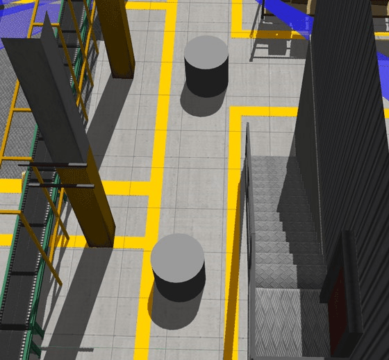
Notice that there are two cylindrical obstacles which are not present on the occupancy map. The robot still avoids them when detected using the VFH algorithm.
A green lamp AvoidingObstacle lights up when the robot is trying to avoid an obstacle.