Plan Path for a Bicycle Robot in Simulink

Open Live Script

This example demonstrates how to execute an obstacle-free path between two locations on a given map in Simulink®. The path is generated using a probabilistic road map (PRM) planning algorithm (mobileRobotPRM). Control commands for navigating this path are generated using the Pure Pursuit controller block. A bicycle kinematic motion model simulates the robot motion based on those commands.

Load the Map and Simulink Model

Load map in MATLAB workspace

load exampleMaps.mat

Enter start and goal locations

startLoc = [5 5];
goalLoc = [12 3];

The imported maps are : simpleMap, complexMap and ternaryMap.

Open the Simulink Model

open_system('pathPlanningBicycleSimulinkModel.slx')

Model Overview

The model is composed of four primary operations :

Planning
Control
Plant Model

Planning

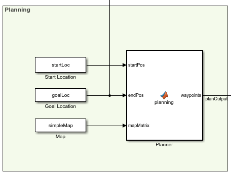
The Planner MATLAB® function block uses the mobileRobotPRM path planner and takes a start location, goal location, and map as inputs. The blocks outputs an array of waypoints that the robot follows. The planned waypoints are used downstream by the Pure Pursuit controller block.

Control

Pure Pursuit

The Pure Pursuit controller block generates the linear velocity and angular velocity commands based on the waypoints and the current pose of the robot.

Check if Goal is Reached

The Check Distance to Goal subsystem calculates the current distance to the goal and if it is within a threshold, the simulation stops.

Plant Model

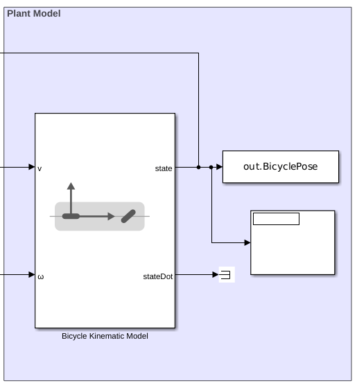
The Bicycle Kinematic Model block creates a vehicle model to simulate simplified vehicle kinematics. The block takes linear and angular velocities as command inputs from the Pure Pursuit controller block, and outputs the current position and velocity states.

Run the Model

To simulate the model

simulation = sim('pathPlanningBicycleSimulinkModel.slx');

Visualize The Motion of Robot

To see the poses :

map = binaryOccupancyMap(simpleMap)

map = 
  binaryOccupancyMap with properties:

   mapLayer Properties
              LayerName: 'binaryLayer'
               DataType: 'logical'
           DefaultValue: 0
    GridLocationInWorld: [0 0]
      GridOriginInLocal: [0 0]
     LocalOriginInWorld: [0 0]
             Resolution: 1
               GridSize: [26 27]
           XLocalLimits: [0 27]
           YLocalLimits: [0 26]
           XWorldLimits: [0 27]
           YWorldLimits: [0 26]

robotPose = simulation.BicyclePose

robotPose = 362×3

    5.0000    5.0000         0
    5.0001    5.0000   -0.0002
    5.0007    5.0000   -0.0012
    5.0036    5.0000   -0.0062
    5.0181    4.9997   -0.0313
    5.0902    4.9929   -0.1569
    5.4081    4.8311   -0.7849
    5.5189    4.6758   -1.1170
    5.5366    4.6356   -1.1930
    5.5512    4.5942   -1.2684
      ⋮

numRobots = size(robotPose, 2) / 3;
thetaIdx = 3;

% Translation
xyz = robotPose;
xyz(:, thetaIdx) = 0;

% Rotation in XYZ euler angles
theta = robotPose(:,thetaIdx);
thetaEuler = zeros(size(robotPose, 1), 3 * size(theta, 2));
thetaEuler(:, end) = theta;

for k = 1:size(xyz, 1)
    show(map)
    hold on;
    
    % Plot Start Location
    plotTransforms([startLoc, 0], eul2quat([0, 0, 0]))
    text(startLoc(1), startLoc(2), 2, 'Start');
    
    % Plot Goal Location
    plotTransforms([goalLoc, 0], eul2quat([0, 0, 0]))
    text(goalLoc(1), goalLoc(2), 2, 'Goal');
    
    % Plot Robot's XY locations
    plot(robotPose(:, 1), robotPose(:, 2), '-b')
    
    % Plot Robot's pose as it traverses the path
    quat = eul2quat(thetaEuler(k, :), 'xyz');
    plotTransforms(xyz(k,:), quat, 'MeshFilePath',...
        'groundvehicle.stl');
    
    pause(0.01)
    hold off;
end