Feedback Control of a ROS-Enabled Robot over ROS 2
This example shows you how to use Simulink® to control a ROS 2 enabled robot running in a Gazebo® robot simulator over ROS 2 network.
Introduction
In this example, you will run a model that implements a simple closed-loop proportional controller. The controller receives location information from a simulated robot and sends velocity commands to drive the robot to a specified location. You will adjust some parameters while the model is running and observe the effect on the simulated robot.
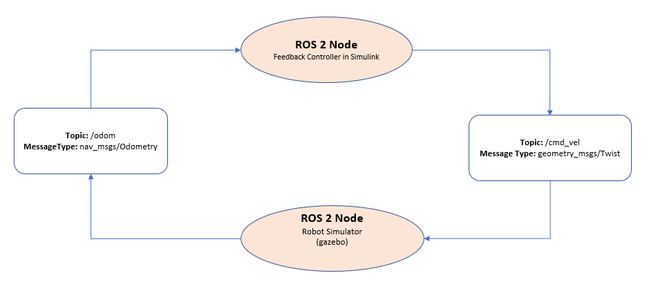
The following diagram summarizes the interaction between Simulink and the robot simulator (the arrows in the diagram indicate ROS 2 message transmission). The /odom topic conveys location information, and the /cmd_vel topic conveys velocity commands.
Prerequisites
To run this example, you are require to set up Docker® in your host environment (Windows Subsystem for Linux (WSL), Linux or Mac) and create a Docker image for Gazebo. For more information on how to configure Docker, see Install and Set Up Docker for ROS, ROS 2, and Gazebo.
Start Docker Container
With the prerequisites set up and the Docker image created, the first step is to launch an instance of Docker container.
To start a Docker container, run the following command in WSL/Linux/Mac terminal:
$ docker run -it --net=host -v /dev/shm:/dev/shm --name ros2_gz_robot <image-name>
Here, 'ros2_gz_robot' is the name of the Docker container. Replace the <image-name> with the name of the Docker image created in the prerequisite section.
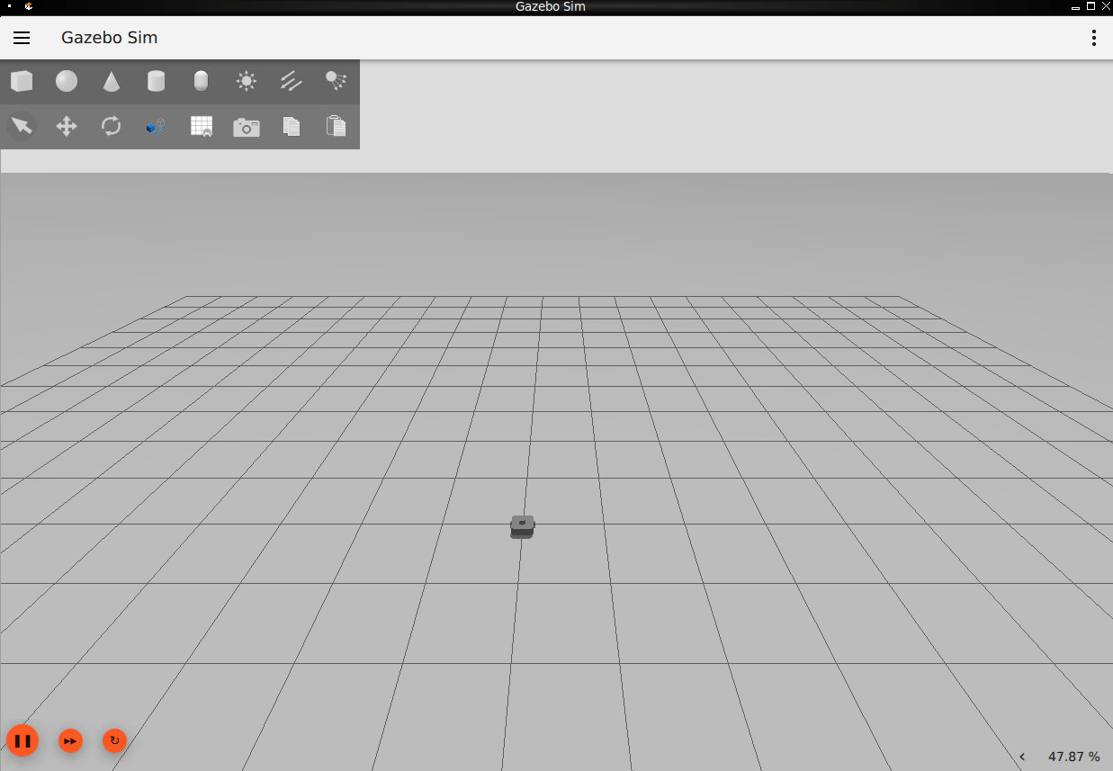
Start Gazebo Robot Simulator
Once the container is running, the next step is to start the Gazebo robot simulator inside the Docker container.
Open a terminal within the Docker container by executing the following command in the WSL/Linux/Mac terminal:
$ docker exec -it ros2_gz_robot /bin/bash
Here, 'ros2_gz_robot' is the docker container name.
In the Docker container terminal, launch the TurtleBot in a Gazebo world by running the following command:
$ source start-gazebo-empty-world.sh
To view the Gazebo world, open a web browser on your Windows® or WSL machine and connect to the URL <docker-ip-address>:8080. If WSL is running on the same host machine, you can simply use localhost:8080. You can now visualize and interact with the Gazebo world directly in your web browser.
Configure MATLAB for ROS 2 Network
Launch MATLAB on your host machine and set the ROS_DOMAIN_ID environment variable to 25 and configure the ROS Middleware in MATLAB to rmw_fastrtps_cpp to match the robot simulator's ROS settings. For detailed steps, refer to Switching Between ROS Middleware Implementations.
Once the domain ID is set, run the following command in MATLAB to verify that the topics from the robot simulator are visible:
setenv('ROS_DOMAIN_ID','25')
ros2 topic list
/camera/camera_info
/camera/image_raw
/camera/image_raw/compressed
/camera/image_raw/compressedDepth
/camera/image_raw/theora
/camera/image_raw/zstd
/clock
/cmd_vel
/imu
/joint_states
/odom
/parameter_events
/robot_description
/rosout
/scan
/tf
/tf_static
The simulator receives and sends messages on the following topics:
Receives
geometry_msgs/Twistvelocity command messages on the /cmd_vel topic.Sends
nav_msgs/Odometrymessages to the/odomtopic.
Open Existing Model
After connecting to the ROS 2 network, open the example model.
open_system('robotROS2FeedbackControlExample.slx');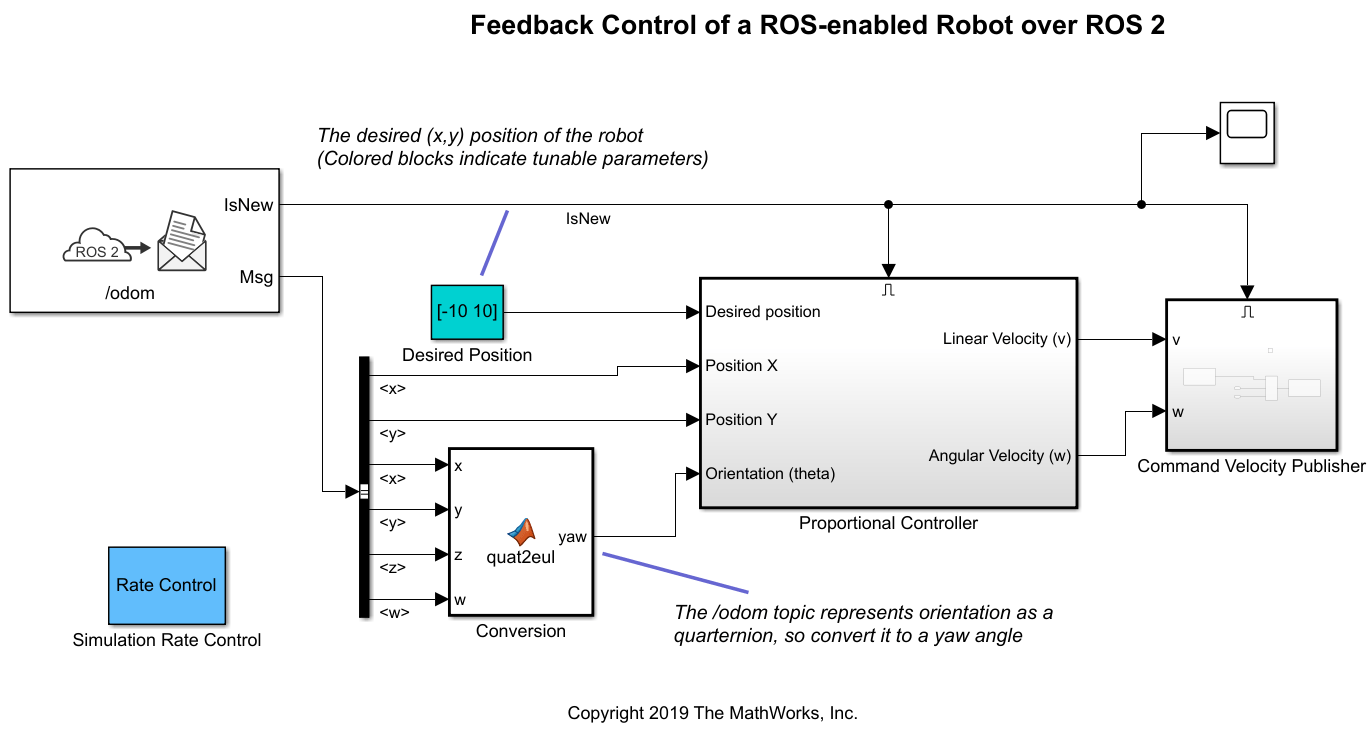
The model implements a proportional controller for a differential-drive mobile robot. On each time step, the algorithm orients the robot toward the desired location and drives it forward. Once the desired location is reached, the algorithm stops the robot.
open_system('robotROS2FeedbackControlExample/Proportional Controller');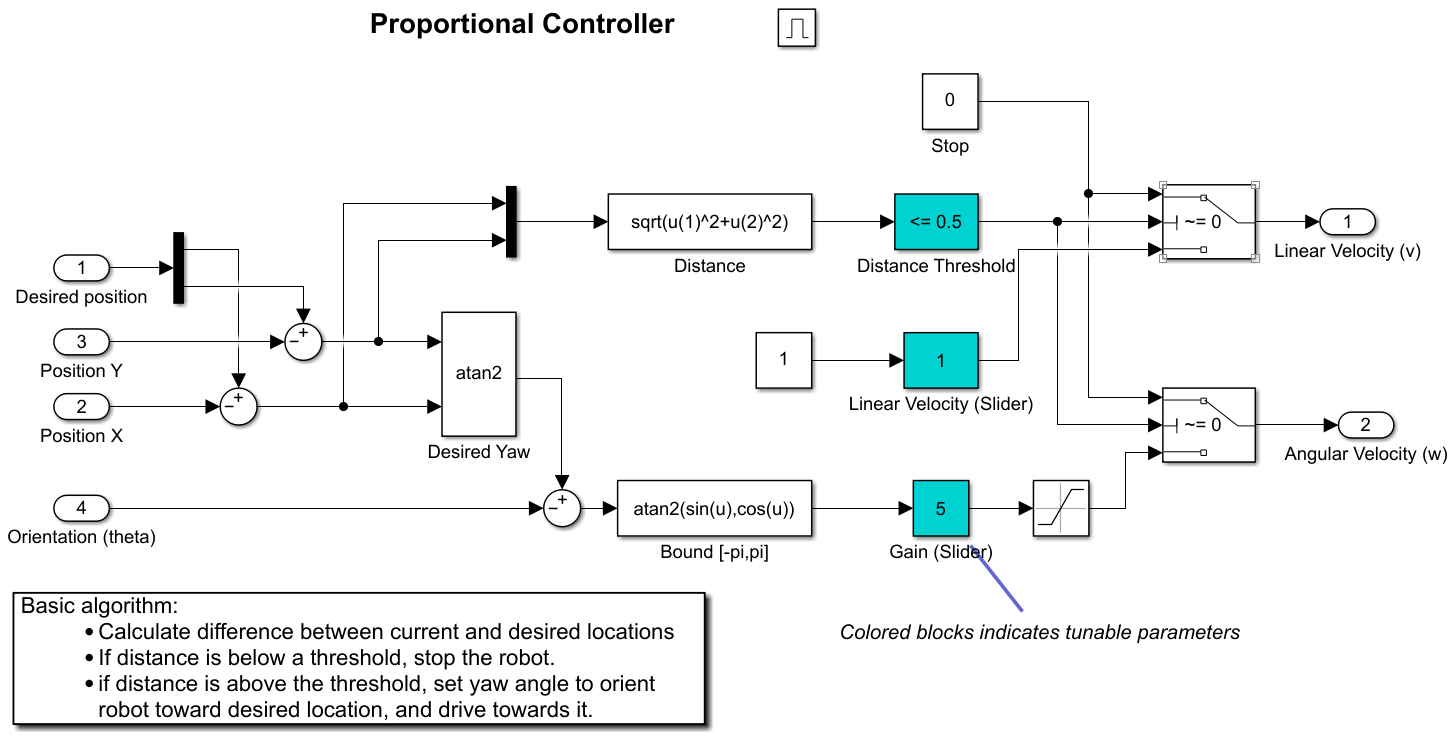
Note that there are four tunable parameters in the model (indicated by colored blocks).
Desired Position (at top level of model): The desired location in (X,Y) coordinates
Distance Threshold: The robot is stopped if it is closer than this distance from the desired location
Linear Velocity: The forward linear velocity of the robot
Gain: The proportional gain when correcting the robot orientation
The model also has a Simulation Rate Control block (at top level of model). This block ensures that the simulation update intervals follow wall-clock elapsed time.
Configure Simulink and Run the Model
In this task, you will configure Simulink to communicate with ROS-enabled robot simulator over ROS 2, run the model and observe the behavior of the robot in the robot simulator.
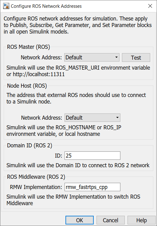
To configure the network settings for ROS 2.
Under the Simulation tab, in PREPARE, select ROS Toolbox > ROS Network.
In Configure ROS Network Addresses, set the ROS 2 Domain ID value to 25.
Make sure the ROS 2 RMW Implementation as
rmw_fastrtps_cpp.Click OK to apply changes and close the dialog box.
To run the model.
Position windows on your screen so that you can observe both the Simulink model and the robot simulator.
Click the Play button in Simulink to start simulation.
While the simulation is running, double-click on the Desired Position block and change the Constant value to
[2 3]. Observe that the robot changes its heading.While the simulation is running, open the Proportional Controller subsystem and double-click on the Linear Velocity (slider) block. Move the slider to 2. Observe the increase in robot velocity.
Click the Stop button in Simulink to stop the simulation.
Observe Rate of Incoming Messages
In this task, you will observe the timing and rate of incoming messages.
Click the Play button in Simulink to start simulation.
Open the Scope block. Observe that the IsNew output of the Subscribe block is always zero, indicating that no messages are being received for the /odom topic. The horizontal axis of the plot indicates simulation time.
Start Gazebo Simulator in ROS network and start ROS Bridge in ROS 2, so that ROS 2 network able receive messages published by Gazebo Simulator.
In the Scope display, observe that the IsNew output has the value 1 at an approximate rate of 20 times per second, in elapsed wall-clock time.
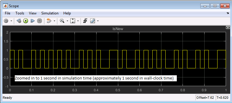
The synchronization with wall-clock time is due to the Simulation Rate Control block. Typically, a Simulink simulation executes in a free-running loop whose speed depends on complexity of the model and computer speed (see Simulation Loop Phase (Simulink) (Simulink)). The Simulation Rate Control block attempts to regulate Simulink execution so that each update takes 0.02 seconds in wall-clock time when possible (this is equal to the fundamental sample time of the model). See the comments inside the block for more information.
In addition, the Enabled subsystems for the Proportional Controller and the Command Velocity Publisher ensure that the model only reacts to genuinely new messages. If enabled subsystems were not used, the model would repeatedly process the same (most-recently received) message over and over, leading to wasteful processing and redundant publishing of command messages.
Clean Up Docker Container
To delete Docker container, run the following command in WSL/Linux/Mac terminal:
$ docker rm ros2_gz_robot
Here, 'ros2_gz_robot' is the name of Docker container.
Summary
This example showed you how to use Simulink for simple closed-loop control of a simulated robot. It also showed how to use Enabled subsystems to reduce overhead in the ROS 2 network.