Find Shortest Control Path in Simulink Model
Model Description
This example shows how to find the shortest control path for a hybrid electrical vehicle using Signal Tracing Command-line API.
To open the model, enter this command in the Command Window.
open_system('sldemo_hevc')
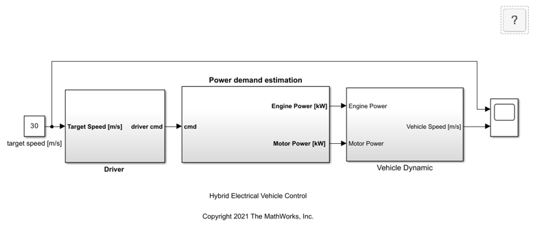
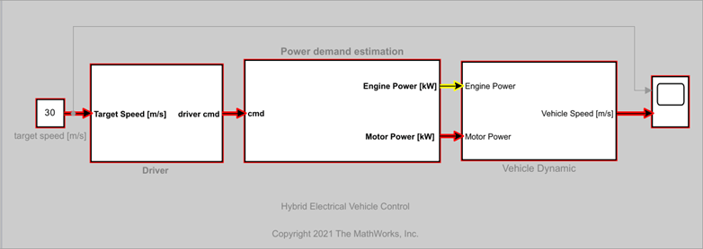
In this model, a hybrid electrical vehicle drives on a slope and the initial speed is 0 m/s. Set the target speed to 30 m/s. In Driver, a PID control compares the actual speed with the target speed and sends a command to increase or decrease speed to the power demand estimation module. Power demand estimation converts to the desired power, and the power is primarily provided by the electrical motor. If electrical motor is unable to provide enough torque, then the engine provides additional torque. In Vehicle Dynamic, road resistance including rolling resistance and gravity resistance as well as the aero drag are calculated. The actual speed of the vehicle is constantly returned to Driver through the feedback loop until the vehicle reaches the target speed.
Trace All Sources That Control the Actual Speed
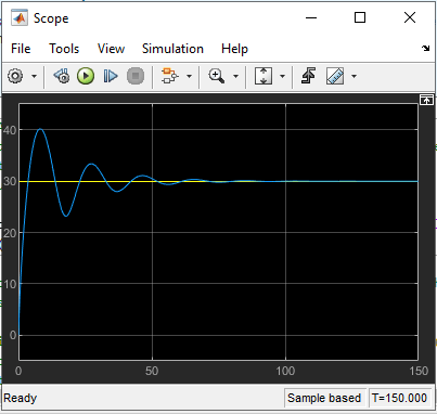
Use the signal tracing API to find the shortest control path to the actual speed. Since the actual speed signal goes into the second inport of Scope, use Scope as the tracing origin.
g = sltrace('sldemo_hevc/Scope', 'source', 'port', '2', 'traceall', 'on');
highlight(g);
Obtain the Trace Graph
The tracing results can be expressed as a MATLAB digraph. The trace graph includes edges and nodes.
A node in trace graph corresponds to a block port in a Simulink® model. The second port of Scope is a node. You can find the node information nodes table.
nodes = g.TraceGraph.Nodes;
The edges are shown as pair of node indexes in trace graph. You can access the node information from the nodes table with the corresponding node index. The Simulink line between nodes is shown as segment handle(s).
edges = g.TraceGraph.Edges;
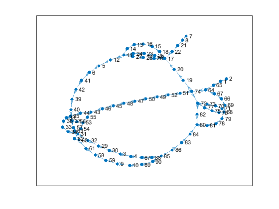
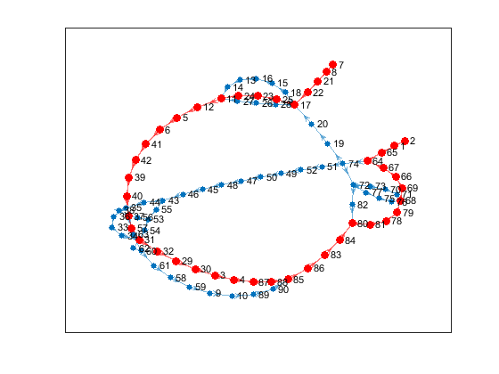
Compute the edges of the trace graph of the sltrace.Graph object and use built-in MATLAB® digraph features to plot the trace graph, as shown in the figure.
fig = g.TraceGraph.plot('Layout', 'force');
Find the Shortest Path from Trace Graph
The start node is the outport of target speed [m/s], and the end node is the second inport of Scope. Use the nodes table to obtain the node indexes of the start node and end node and compute the shortest path between them, as shown in the figure.
startNode = 7;
endNode = 2;
shortestPath = g.TraceGraph.shortestpath(startNode, endNode);
highlight(fig, shortestPath, 'EdgeColor','r','NodeColor','r','MarkerSize',6,'LineWidth',1);
Find the Shortest Control Path from the Simulink Model
The edges table contains two types of edges: real edges and virtual edges, including internal edges and hidden edges. First, filter out the virtual edges using the MATLAB find function.
realEdgeIdx = find(cellfun(@(x) ~ischar(x), edges.Segments) == 1);
realEdges = edges(realEdgeIdx, :);
Process each node in the shortest path to obtain the corresponding blocks and segments. Since one source node may be connected to multiple destination nodes, iterate over all the edges from the same source node and find the target destination node on the shortest path.
elements = [];
for i = 1:length(shortestPath) - 1
    srcNodeIdx = shortestPath(i);
    dstNodeIdx = shortestPath(i+1);
    srcBlockHandle = nodes.Block(srcNodeIdx);
    srcNodeEdgeIdx = find(realEdges.EndNodes(:,2) == dstNodeIdx);
    if length(srcNodeEdgeIdx) > 1
       dstNodeEdgeIdx = find(realEdges.EndNodes(srcNodeEdgeIdx, 2) == dstNodeIdx) ;
       edgeIdx = srcNodeEdgeIdx(dstNodeEdgeIdx);
    elseif length(srcNodeEdgeIdx) == 1
        edgeIdx = srcNodeEdgeIdx;
    else
        continue;
    end
    elements = [elements srcBlockHandle flip(realEdges.Segments{edgeIdx})];
end
Process the last node in the shortest path and highlight the shortest path in the Simulink model, as shown in the figure.
lastNodeIdx = shortestPath(end);
lastBlockHandle = nodes.Block(lastNodeIdx);
elements = [elements lastBlockHandle];
highlight(g, elements)