Solve Algebraic Loops as Differential-Algebraic Equations (DAEs)

R2026b

This example shows how to solve the algebraic loop in a practical drivetrain model as a differential-algebraic equation (DAE). The example compares the DAE approach to the algebraic loop solver and explains how to decide when to use each option.

Open Drivetrain Model

Open the drivetrain model. The model represents a motor driving a load through two flexible shaft segments joined by a bolted flange. The bolted flange introduces rigid coupling between the motor shaft and load shaft.

mdl = "DrivetrainDAE";
open_system(mdl)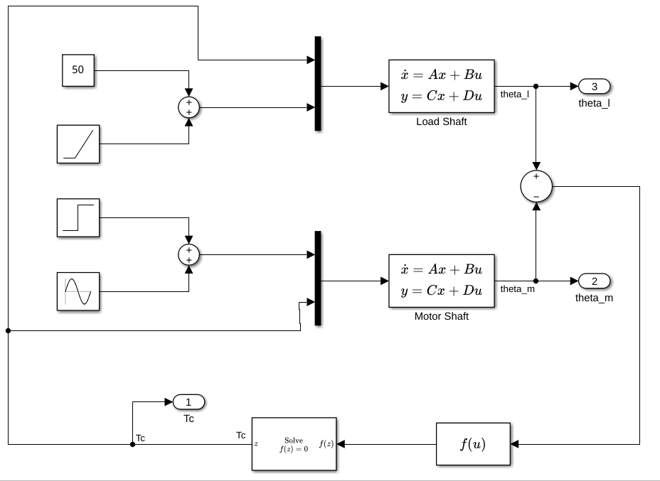

Block diagram of the model DrivetrainDAE.

The model contains:

Two State-Space blocks that represent Craig-Bampton reduced shaft substructures for the motor and load
An Algebraic Constraint block that solves for the coupling torque $T_{c}$
A summation that computes the interface displacement difference
A nonlinear coupling block that implements the hardening spring behavior
Feedback paths that carry $T_{c}$ back to both State-Space blocks

Algebraic Loop in the Drivetrain Model

Each shaft substructure is expressed in state-space form after Craig-Bampton component mode synthesis (CMS) reduction. The state-space equations for the motor-side shaft are:

${x_{}^{˙}}_{m} = A_{m} x_{m} + B_{m} u_{m}$

$θ_{m} = C_{m} x_{m} + D_{m} u_{m}$

The load-side shaft has an analogous form. The critical feature is the interface compliance in the $D$ matrices. CMS static condensation produces a non-zero direct feedthrough matrix ( $D \neq 0$ ). This means the outputs $θ_{m}$ and $θ_{l}$ depend immediately on the coupling torque $T_{c}$ , not just through integration.

At the rigid coupling, the interface displacements must satisfy a nonlinear constraint:

$f (Δ θ) = Δ θ + 200 (Δ θ)^{3} = 0$

where $Δ θ = θ_{m} - θ_{l}$ . The Algebraic Constraint block solves for $T_{c}$ such that this constraint holds at every time step.

The algebraic loop forms because of the circular dependency. The Algebraic Constraint block produces $T_{c}$ , which feeds into both State-Space blocks. Due to $D \neq 0$ , the outputs $θ_{m}$ and $θ_{l}$ immediately depend on $T_{c}$ , and their difference feeds back into the Algebraic Constraint block.

Simulate Using Algebraic Loop Solver

By default, Simulink solves the algebraic loop using the algebraic loop solver. In each time step, the algebraic loop solver iteratively solves the loop. In each iteration, the solver:

Evaluates the loop by guessing the value of $T_{c}$
Checks whether the solution converged
Updates the guess for $T_{c}$ if the solution did not converge

Each iteration executes all the blocks in the algebraic loop. The algebraic loop solver can take several iterations to find a solution.

Configure the Algebraic Constraint block to solve the loop using the algebraic loop solver. Then, simulate the model.

set_param(mdl + "/Algebraic Constraint", ...
    EquationFormat="Algebraic Loop")

outAlgLoop = sim(mdl);

Simulate by Solving Loop as DAE

Instead of iterating on the algebraic loop at each step, the constraint can be absorbed into the differential equation system. The implicit ODE solver (ode23t) handles the differential and algebraic equations simultaneously as a single system. The algebraic constraint is satisfied as part of the solver's own Newton iteration, eliminating the need to use a separate algebraic loop solver at most time steps. The algebraic loop solver is used at the beginning of the simulation and at zero crossing events to compute consistent initial conditions for the ODE solver.

Configure the Algebraic Constraint block to solve the loop using as a DAE. Then, simulate the model.

set_param(mdl + "/Algebraic Constraint", ...
    EquationFormat="Differential Algebraic Equation")

outDAE = sim(mdl);

When does solving as a DAE help most?

Models where the algebraic loop requires many iterations per step (ill-conditioned loops, nonlinear constraints)
Models with expensive block evaluations inside the loop
Long simulations where per-step savings accumulate

Solving as a DAE requires an implicit solver and continuous sample time for the algebraic loop. For very simple loops with fast convergence, the performance improvement may be minimal.

Analyze Simulation Results

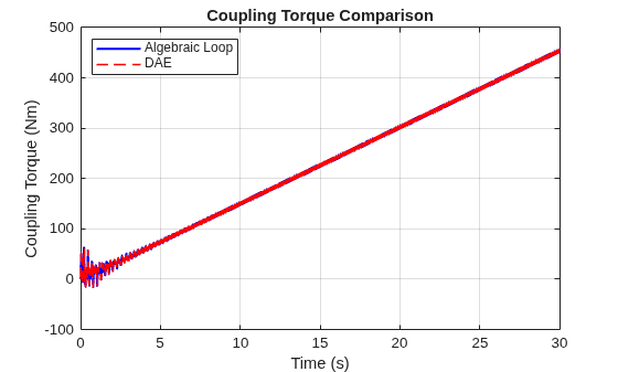
Both approaches produce numerically equivalent results within solver tolerance. Compare the coupling torque from the two simulations to verify equivalence.

figure
plot(outAlgLoop.yout.get("Tc").Values.Time, outAlgLoop.yout.get("Tc").Values.Data, "b", LineWidth=1.5)
hold on
plot(outDAE.yout.get("Tc").Values.Time, outDAE.yout.get("Tc").Values.Data, "r--", LineWidth=1.2)
legend("Algebraic Loop", "DAE", Location="northwest")
xlabel("Time (s)")
ylabel("Coupling Torque (Nm)")
title("Coupling Torque Comparison")
grid on

Figure contains an axes object. The axes object with title Coupling Torque Comparison, xlabel Time (s), ylabel Coupling Torque (Nm) contains 2 objects of type line. These objects represent Algebraic Loop, DAE.