Enforce Lyapunov Stability for Adaptive Cruise Control

R2026b

This example uses:

This example shows how to use the Control Lyapunov Function block to enforce stability for adaptive cruise control (ACC), and optionally combine it with barrier certificate constraints for safety.

Overview

In this example, the goal is to make an ego car travel at a set velocity while maintaining a safe distance from a lead car. The Control Lyapunov Function (CLF) block enforces exponential convergence of velocity to the desired speed. When combined with a control barrier function (CBF), the system simultaneously guarantees stability (CLF) and safety (CBF).

Configure model parameters.

x0_lead = 50;         % Initial position for lead car (m)
v0_lead = 25;         % Initial velocity for lead car (m/s)
x0_ego = 10;          % Initial position for ego car (m)
v0_ego = 20;          % Initial velocity for ego car (m/s)
default_spacing = 10; % Default spacing (m)
time_gap = 1.4;       % Time gap (s)
v_set = 28;           % Driver-set velocity (m/s)
min_ac = -3;          % Minimum acceleration for driver comfort (m/s^2)
max_ac = 2;           % Maximum acceleration for driver comfort (m/s^2)
Ts = 0.1;             % Sample time (s)
T = 80;               % Duration (s)

The lead car has a time-varying acceleration profile that produces braking and acceleration phases. The resulting velocity transitions from 25 m/s down to 18 m/s and back, which better demonstrates the CLF's ability to guarantee exponential convergence to the desired velocity.

a_lead_time = [0 14.99 15 29.99 30 44.99 45 59.99 60 T];
a_lead_val = [0 0 -7/15 -7/15 0 0 7/15 7/15 0 0];

Open the model.

mdl = "lyapunovStabilityACC";
open_system(mdl)

Control Lyapunov Function for Velocity Tracking

The vehicle dynamics are described by the following equations.

$p_{}^{˙} = v$

$v_{}^{˙} = u$

$d_{}^{˙} = v_{l} - v$

Here, $p$ is the position of the ego car, $v$ is its velocity, $d$ is the relative distance, and $v_{l}$ is the velocity of the lead car. The control input $u$ is the acceleration of the ego car.

The Control Lyapunov Function block accepts plant dynamics in the form $x_{}^{˙} = f (x) + g (x) u$ . For this application, $f (x) = [\begin{array}{c} v \\ 0 \\ v_{l} - v \end{array}]$ and $g (x) = [\begin{array}{c} 0 \\ 1 \\ 0 \end{array}]$ , where state variables are $x = [\begin{array}{c} p \\ v \\ d \end{array}]$ .

Lyapunov Function

The control objective is to track the desired velocity $v_{d}$ . The Lyapunov function is chosen as $V (x) = (v - v_{d})^{2}$ , which is zero when the ego car travels at the desired speed and positive otherwise.

The gradient of $V$ with respect to the states is $\frac{\partial V}{\partial x} = [\begin{array}{ccc} 0 & 2 (v - v_{d}) & 0 \end{array}]$ .

The CLF constraint enforces:

$\frac{\partial V}{\partial x} (f (x) + g (x) u) + c V (x) \leq δ$

where $c > 0$ is the CLF rate that controls the exponential convergence speed, and $δ \geq 0$ is a relaxation variable.

The nominal control is set to zero ( $u_{nom} = 0$ ), so the CLF block generates the minimum control effort needed to achieve exponential convergence.

CLF Parameters

The CLF rate $c$ determines how aggressively the velocity converges to the desired value. A larger $c$ means faster convergence but potentially larger control effort. The relaxation penalty weight $p$ determines how strongly the QP penalizes relaxation of the CLF constraint, as shown in the cost function:

$J = \frac{1}{2} (| u - u_{0} |^{2} + p δ^{2})$

clf_rate = 0.5;        % CLF convergence rate
penalty_weight = 10;   % Relaxation penalty weight

Simulate CLF-Only Controller

First, simulate with the CLF constraint only (no barrier certificate). This simulation demonstrates that the CLF guarantees exponential convergence of velocity to the desired speed.

use_cbf = 0;
sim(mdl);
accCLFPlotResults(logsout,default_spacing,time_gap,v_set, ...
"CLF Only (No Safety Constraint)")

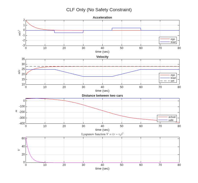
The Lyapunov function $V = (v - v_{d})^{2}$ converges exponentially toward zero, demonstrating that the CLF block successfully enforces stability. However, without a safety constraint, the ego car may violate the safe following distance. The third plot in the above figure shows that the actual distance between cars is less than safe distance.

Adding Barrier Certificate for Safety

The safety set is defined as the relative distance $d \geq d_{safe}$ , where $d_{safe} = τ v + d_{0}$ . The barrier certificate is $h (x) = d - τ v - d_{0} \geq 0$ , with gradient $\frac{\partial h}{\partial x} = [\begin{array}{ccc} 0 & - τ & 1 \end{array}]$ .

When the CLF and CBF constraints conflict (the ego car wants to go faster but needs to maintain safe distance), the CLF constraint is relaxed via the $δ$ variable while the CBF constraint remains hard. This ensures safety is never violated while stability is achieved whenever possible.

Simulate CLF+CBF Controller

Enable the barrier certificate constraint and re-simulate.

use_cbf = 1;
sim(mdl);
accCLFPlotResults(logsout,default_spacing,time_gap,v_set, ...
"CLF + CBF (Stability and Safety)")

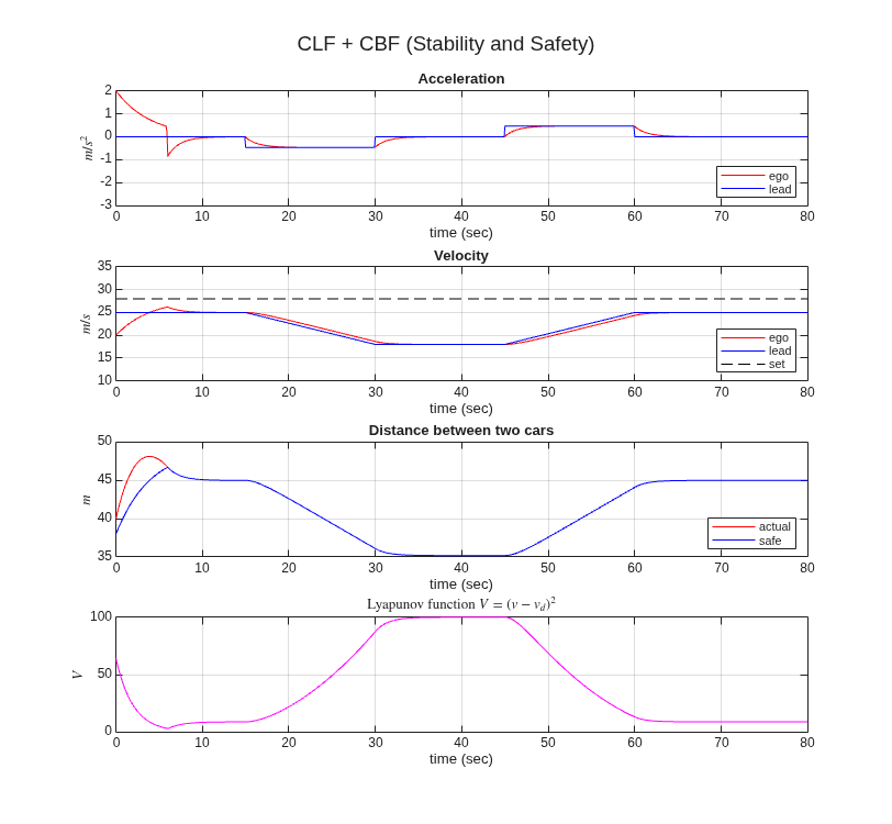
The results show that:

The barrier certificate (safety offset) remains nonnegative at all times, guaranteeing safety.
The Lyapunov function still converges when the CLF and CBF do not conflict (the ego car can track the desired velocity while maintaining safe distance).
When the lead car brakes and the safe distance is threatened, the CLF constraint relaxes to prioritize safety, and the ego car slows down.
Once the lead car accelerates and sufficient headway is restored, the CLF resumes driving the velocity toward the desired value.

The Control Lyapunov Function block, combined with a control barrier function, provides a principled QP-based approach to simultaneously guarantee stability (velocity tracking) and safety (collision avoidance) for adaptive cruise control.