Train Reinforcement Learning Agent with Constraint Enforcement
This example shows how to train a reinforcement learning (RL) agent with actions constrained using the Constraint Enforcement block. This block computes modified control actions that are closest to the actions output by the agent subject to constraints and action bounds. Training reinforcement learning agents requires Reinforcement Learning Toolbox™ software.
In this example, the goal of the agent is to bring a green ball as close as possible to the changing target position of a red ball [1].
The dynamics for the green ball from velocity to position are governed by Newton's law with a small damping coefficient :
The feasible region for the ball position and the velocity of the green ball is limited to the range .
The position of the target red ball is uniformly random across the range . The agent can observe only a noisy estimate of this target position.
Set the random seed to ensure reproducibility.
rng("default")Configure model parameters.
Tv = 0.8;            % sample time for visualizer
Ts = 0.1;            % sample time for controller
tau = 0.01;          % damping constant for green ball
velLimit = 1;        % maximum speed for green ball
s0 = 200;            % random seed
s1 = 100;            % random seed
x0 = 0.2;            % initial position for ball
Create Environment and Agent for Collecting Data
In this example, a constraint function is represented using a trained deep neural network. To train the network, you must first collect training data from the environment.
To do so, first create an RL environment using the rlBallOneDim model. This model applies random external actions through an RL Agent block to the environment.
mdl = "rlBallOneDim";
open_system(mdl)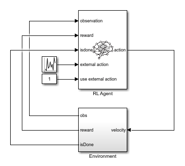
The Environment subsystem performs the following steps.
Applies the input velocity to the environment model and generates the resulting output observations
Computes the training reward , where denotes the position of the red ball
Sets the termination signal
isDonetotrueif the ball position violates the constraint
For this model, the observations from the environment include the position and velocity of the green ball and the noisy measurement of the red ball position. Define a continuous observation space for these three values.
obsInfo = rlNumericSpec([3 1]);
The action that the agent applies to the green ball is its velocity. Create a continuous action space and apply the required velocity limits.
actInfo = rlNumericSpec([1 1], ...
    LowerLimit=-velLimit, ...
    UpperLimit=velLimit);
Create an RL environment for this model.
agentblk = mdl + "/RL Agent";
env = rlSimulinkEnv(mdl,agentblk,obsInfo,actInfo);
Specify a reset function, which randomly initializes the environment at the start of each training episode or simulation.
env.ResetFcn = @(in)localResetFcn(in);
Next, create a DDPG reinforcement learning agent, which supports continuous actions and observations, using the createDDPGAgentBall helper function. This function creates critic and actor representations based on the action and observation specifications and uses the representations to create a DDPG agent.
agent = createDDPGAgentBall(Ts,obsInfo,actInfo);
In the rlBallOneDim model, the RL Agent block does not generate actions. Instead, it is configured to pass a random external action to the environment. The purpose for using a data-collection model with an inactive RL Agent block is to ensure that the environment model, action and observation signal configurations, and model reset function used during data collection match those used during subsequent agent training.
Learn Constraint Function
In this example, the ball position signal must satisfy . To allow for some slack, the constraint is set to be The dynamic model from velocity to position has a very small damping constant, thus it can be approximated by . Therefore, the constraints for green ball are given by the following equation.
The Constraint Enforcement block accepts constraints of the form . For the above equation, the coefficients of this constraint function are as follows.
The function is approximated by a deep neural network that is trained on the data collected by simulating the RL agent within the environment. To learn the unknown function , the RL agent passes a random external action to the environment that is uniformly distributed in the range .
To collect data, use the collectDataBall helper function. This function simulates the environment and agent and collects the resulting input and output data. The resulting training data has three columns: , , and .
For this example, load precollected training data. To collect the data yourself, set collectData to true.
collectData = false;
if collectData
    count = 1050;
    data = collectDataBall(env,agent,count);
else
    load("trainingDataBall.mat","data")
end
Train a deep neural network to approximate the constraint function using the trainConstraintBall helper function. This function formats the data for training then creates and trains a deep neural network. Training a deep neural network requires Deep Learning Toolbox™ software.
For this example, to ensure reproducibility, load a pretrained network. To train the network yourself, set trainConstraint to true.
trainConstraint = false;
if trainConstraint
    network = trainConstraintBall(data);
else
    load("trainedNetworkBall.mat","network")
end
The following figure shows an example of the training progress.
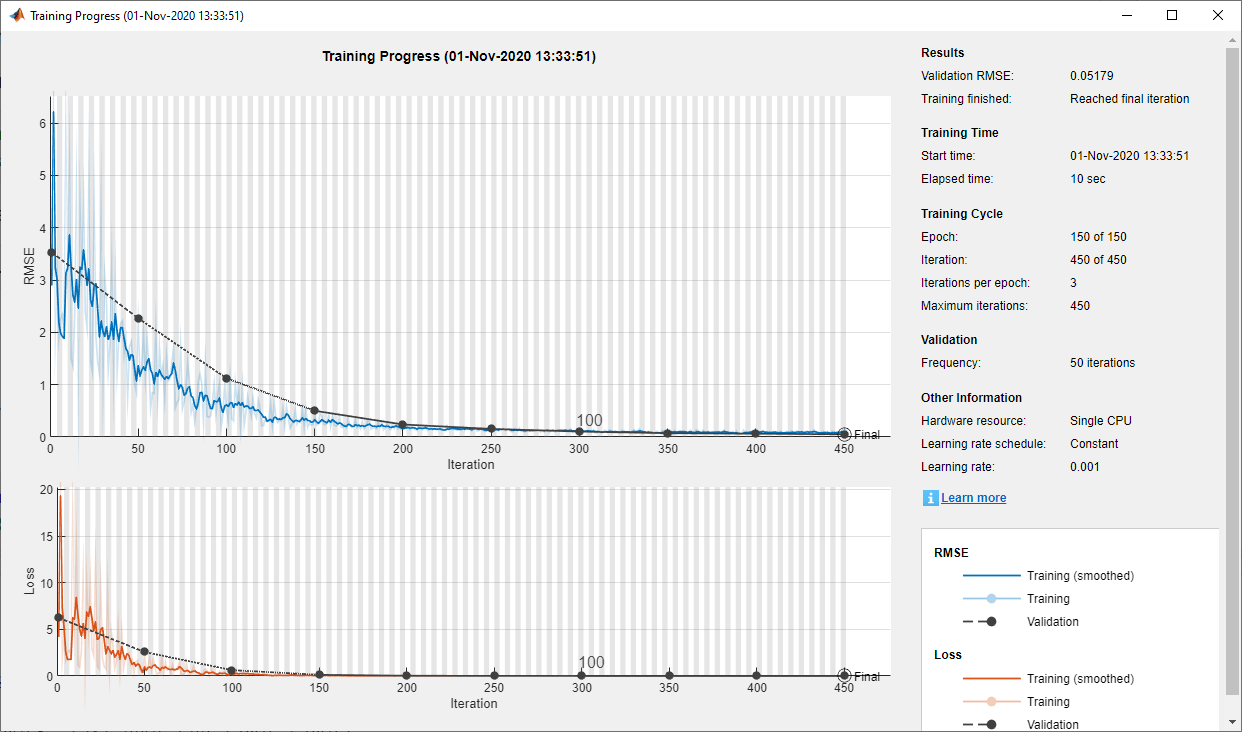
Validate the trained neural network using the validateNetworkBall helper function. This function processes the input training data using the trained deep neural network. It then compares the network output with the training output and computes the root mean-squared error (RMSE).
validateNetworkBall(data,network)
Test Data RMSE = 9.100315e-02
The small RMSE value indicates that the network successfully learned the constraint function.
Train Agent with Constraint Enforcement
To train the agent with constraint enforcement, use the rlBallOneDimWithConstraint model. This model constrains the actions from the agent before applying them to the environment.
mdl = "rlBallOneDimWithConstraint";
open_system(mdl)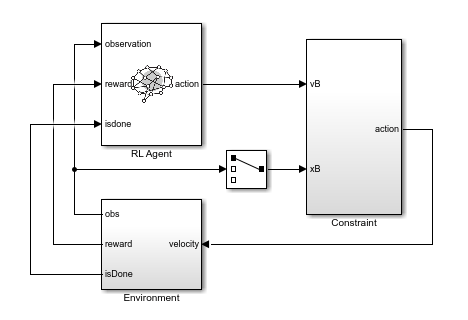
To view the constraint implementation, open the Constraint subsystem. Here, the trained deep neural network approximates , and the Constraint Enforcement block enforces the constraint function and velocity bounds.
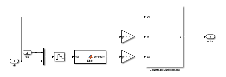
For this example the following Constraint Enforcement block parameter settings are used.
Number of constraints —
2Number of actions —
1Constraint bound —
[0.9;-0.1]
Create an RL environment using this model. The observation and action specifications match those used for the previous data collection environment.
agentblk = mdl + "/RL Agent";
env = rlSimulinkEnv(mdl,agentblk,obsInfo,actInfo);
env.ResetFcn = @(in)localResetFcn(in);
Specify options for training the agent. Train the RL agent for 120 episodes with 300 steps per episode.
trainOpts = rlTrainingOptions(...
    MaxEpisodes=120, ...
    MaxStepsPerEpisode=300, ...
    Verbose=false, ...
    Plots="training-progress");
Train the agent. Training is a time-consuming process. For this example, load a pretrained agent. To train the agent yourself, set trainAgent to true.
trainAgent = false;
if trainAgent
    trainingStats = train(agent,env,trainOpts);
else
    load("rlAgentBallParams.mat","agent")
end
The following figure shows the training results. The training process converges to a good agent within 40 episodes.
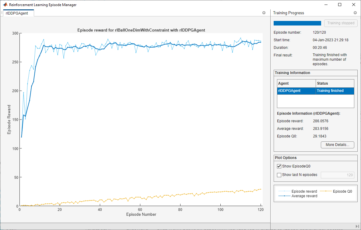
Since Total Number of Steps equals the product of Episode Number and Episode Steps, each training episode runs to the end without early termination. Therefore, the Constraint Enforcement block ensures that the ball position never violates the constraint .
Simulate the trained agent using the simWithTrainedAgentBall helper function.
simWithTrainedAgentBall(env,agent)

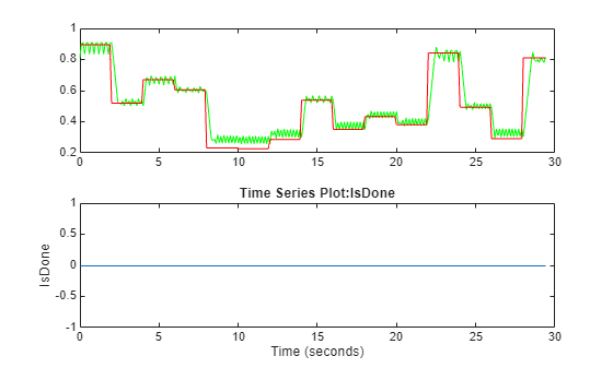
The agent successfully tracks the position of the red ball.
Train Agent Without Constraint Enforcement
To see the benefit of training an agent with constraint enforcement, you can train the agent without constraints and compare the training results to the constraint enforcement case.
To train the agent without constraints, use the rlBallOneDimWithoutConstraint model. This model applies the actions from the agent directly to the environment.
mdl = "rlBallOneDimWithoutConstraint";
open_system(mdl)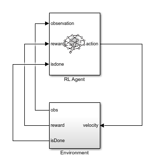
Create an RL environment using this model.
agentblk = mdl + "/RL Agent";
env = rlSimulinkEnv(mdl,agentblk,obsInfo,actInfo);
env.ResetFcn = @(in)localResetFcn(in);
Create a new DDPG agent to train. This agent has the same configuration as the agent used in the previous training.
agentNoConstraint = createDDPGAgentBall(Ts,obsInfo,actInfo);
Train the agent using the same training options as in the constraint enforcement case. For this example, as with the previous training, load a pretrained agent. To train the agent yourself, set trainAgent to true.
trainAgent = false;
if trainAgent
    trainingStats2 = train(agentNoConstraint,env,trainOpts);
else
    load("rlAgentBallCompParams.mat","agentNoConstraint")
end
The following figure shows the training results. The training process converges to a good agent after about 90 episodes.
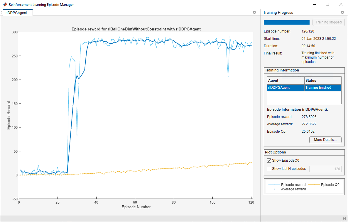
Since Total Number of Steps is less than the product of Episode Number and Episode Steps, the training includes episodes that terminated early due to constraint violations.
Simulate the trained agent.
simWithTrainedAgentBall(env,agentNoConstraint)

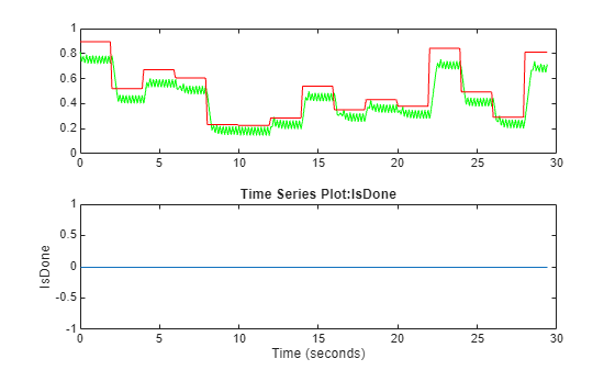
The agent tracks the position of the red ball with more steady-state offset than the agent trained with constraints.
Conclusion
In this example, training an RL agent with the Constraint Enforcement block ensures that the actions applied to the environment never produce a constraint violation. As a result, the training process converges to a good agent quickly. Training the same agent without constraints produces slower convergence and poorer performance.
close("Ball One Dim")Local Reset Function
function in = localResetFcn(in)
% Reset function
in = setVariable(in,"x0",rand);
in = setVariable(in,"s0",randi(5000));
in = setVariable(in,"s1",randi(5000));
end
References
[1] Dalal, Gal, Krishnamurthy Dvijotham, Matej Vecerik, Todd Hester, Cosmin Paduraru, and Yuval Tassa. "Safe Exploration in Continuous Action Spaces." Preprint, submitted January 26, 2018. https://arxiv.org/abs/1801.08757
See Also
Blocks
- Constraint Enforcement | RL Agent (Reinforcement Learning Toolbox)