Inductor with Hysteresis

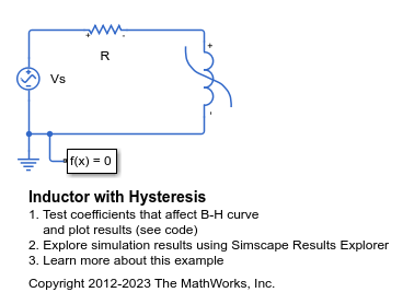
This example shows how modifying the equation coefficients of the Jiles-Atherton magnetic hysteresis equations affects the resulting B-H curve. The simulation parameters are configured to run four complete AC cycles with initial field strength (H) and magnetic flux density (B) both set to zero.

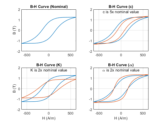
Parameters that set the shape of the anhysteretic curve are not perturbed as selecting values for these parameters is relatively easy. The remaining three parameters affect the B-H curve in multiple ways, and some iteration is typically needed to match a nominal B-H curve. The following steps are a good starting point:

1. Tune c to match the initial gradient when starting at B=H=0. As c approaches 1 the gradient will match that of the anhysteretic curve. Making it smaller reduces the initial gradient.

2. Tune K to get the desired H-axis intercepts. A good initial guess for K is the actual value of the desired intercept.

3. Gradually increase alpha (starting from a value like 1e-6) to fine tune the B-axis intercepts. Making alpha bigger increases the intercept values.

Model

Simulation Results from Simscape Logging

The plots below show how the individual Jiles-Atherton hysteresis coefficients affect the hysteresis curve for a nonlinear inductor. The model is simulated with a nominal set of Jiles-Atherton hysteresis equation coefficients, and then re-runs the model with perturbations applied to each coefficient individually.