binocdf
Binomial cumulative distribution function
Description
y = binocdf(x,n,p)x using the corresponding number of trials in n
and the probability of success for each trial in p.
x, n, and p can be
vectors, matrices, or multidimensional arrays of the same size. Alternatively, one or more
arguments can be scalars. The binocdf function expands scalar inputs to
constant arrays with the same dimensions as the other inputs.
Examples
Compute and plot the binomial cumulative distribution function for the specified range of integer values, number of trials, and probability of success for each trial.
A baseball team plays 100 games in a season and has a 50-50 chance of winning each game. Find the probability of the team winning more than 55 games in a season.
format long
1 - binocdf(55,100,0.5)
ans = 0.135626512036917
Find the probability of the team winning between 50 and 55 games in a season.
binocdf(55,100,0.5) - binocdf(49,100,0.5)
ans =
   0.404168106656672
Compute the probabilities of the team winning more than 55 games in a season if the chance of winning each game ranges from 10% to 90%.
chance = 0.1:0.05:0.9;
y = 1 - binocdf(55,100,chance);
Plot the results.
scatter(chance,y)
grid on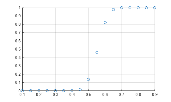
Compute the complement of the binomial cumulative distribution function with more accurate upper tail probabilities.
A baseball team plays 100 games in a season and has a 50-50 chance of winning each game. Find the probability of the team winning more than 95 games in a season.
format long
1 - binocdf(95,100,0.5)
ans =
0
This result shows that the probability is so close to 1 (within eps) that subtracting it from 1 gives 0. To approximate the extreme upper tail probabilities better, compute the complement of the binomial cumulative distribution function directly instead of computing the difference.
binocdf(95,100,0.5,'upper')ans =
3.224844447881779e-24
Alternatively, use the binopdf function to find the probabilities of the team winning 96, 97, 98, 99, and 100 games in a season. Find the sum of these probabilities by using the sum function.
sum(binopdf(96:100,100,0.5),'all')ans =
3.224844447881779e-24
Input Arguments
Output Arguments
More About
Alternative Functionality
binocdfis a function specific to binomial distribution. Statistics and Machine Learning Toolbox™ also offers the generic functioncdf, which supports various probability distributions. To usecdf, specify the probability distribution name and its parameters. Alternatively, create aBinomialDistributionprobability distribution object and pass the object as an input argument. Note that the distribution-specific functionbinocdfis faster than the generic functioncdf.Use the Probability Distribution Function Tool to create an interactive plot of the cumulative distribution function (cdf) or probability density function (pdf) for a probability distribution.
Extended Capabilities
Version History
Introduced before R2006a