geocdf
Geometric cumulative distribution function
Description
Examples
Compute Geometric Distribution cdf
Toss a fair coin repeatedly until the coin successfully lands with heads facing up. Determine the probability of observing at most three tails before tossing heads.
Compute the value of the cumulative distribution function (cdf) for the geometric distribution evaluated at the point x = 3
, where x
is the number of tails observed before the result is heads. Because the coin is fair, the probability of getting heads in any given toss is p = 0.5
.
x = 3; p = 0.5; y = geocdf(x,p)
y = 0.9375
The returned value y
indicates that the probability of observing three or fewer tails before tossing heads is 0.9375.
Compute Multiple Geometric Distribution cdfs
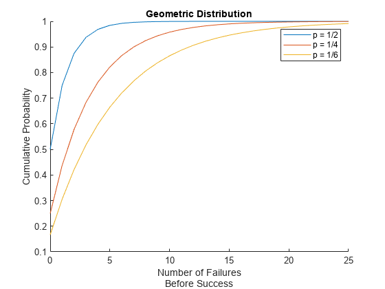
Compare the cumulative distribution functions (cdfs) of three geometric distributions.
Create a probability vector that contains three different parameter values.
The first parameter corresponds to a geometric distribution that models the number of times you toss a coin before the result is heads.
The second parameter corresponds to a geometric distribution that models the number of times you roll a four-sided die before the result is a 4.
The third parameter corresponds to a geometric distribution that models the number of times you roll a six-sided die before the result is a 6.
p = [1/2 1/4 1/6]'
p = 3×1
0.5000
0.2500
0.1667
For each geometric distribution, evaluate the cdf at the points x
= 0,1,2,...,25. Expand x
and p
so that the two geocdf
input arguments have the same dimensions.
x = 0:25
x = 1×26
0 1 2 3 4 5 6 7 8 9 10 11 12 13 14 15 16 17 18 19 20 21 22 23 24 25
expandedX = repmat(x,3,1); expandedP = repmat(p,1,26); y = geocdf(expandedX,expandedP)
y = 3×26
0.5000 0.7500 0.8750 0.9375 0.9688 0.9844 0.9922 0.9961 0.9980 0.9990 0.9995 0.9998 0.9999 0.9999 1.0000 1.0000 1.0000 1.0000 1.0000 1.0000 1.0000 1.0000 1.0000 1.0000 1.0000 1.0000
0.2500 0.4375 0.5781 0.6836 0.7627 0.8220 0.8665 0.8999 0.9249 0.9437 0.9578 0.9683 0.9762 0.9822 0.9866 0.9900 0.9925 0.9944 0.9958 0.9968 0.9976 0.9982 0.9987 0.9990 0.9992 0.9994
0.1667 0.3056 0.4213 0.5177 0.5981 0.6651 0.7209 0.7674 0.8062 0.8385 0.8654 0.8878 0.9065 0.9221 0.9351 0.9459 0.9549 0.9624 0.9687 0.9739 0.9783 0.9819 0.9849 0.9874 0.9895 0.9913
Each row of y
contains the cdf values for one of the three geometric distributions.
Compare the three geometric distributions by plotting the cdf values.
hold on plot(x,y(1,:)) plot(x,y(2,:)) plot(x,y(3,:)) legend(["p = 1/2","p = 1/4","p = 1/6"]) xlabel(["Number of Failures","Before Success"]) ylabel("Cumulative Probability") title("Geometric Distribution") hold off
Compute Complement of Geometric Distribution cdf
Roll a fair die repeatedly until you successfully get a 6. Determine the probability of failing to roll a 6 within the first three rolls.
Compute the complement of the cumulative distribution function (cdf) for the geometric distribution evaluated at the point x = 2
, where x
is the number of non-6 rolls before the result is a 6. Note that an x
value of 2 or less indicates successfully rolling a 6 within the first three rolls. Because the die is fair, the probability of getting a 6 in any given roll is p = 1/6
.
x = 2;
p = 1/6;
y = geocdf(x,p,"upper")
y = 0.5787
The returned value y
indicates that the probability of failing to roll a 6 within the first three rolls is 0.5787. Note that this probability is equal to the probability of rolling a non-6 value three times.
probability = (1-p)^3
probability = 0.5787
Input Arguments
x
— Values at which to evaluate cdf
nonnegative integer scalar | array of nonnegative integer scalars
Values at which to evaluate the cdf, specified as a nonnegative integer scalar or an array of nonnegative integer scalars.
To evaluate the cdf at multiple values, specify x
using an
array. To evaluate the cdfs of multiple distributions, specify p
using an array. If both of the input arguments x
and
p
are arrays, then the array sizes must be the same. If only one
of the input arguments is an array, then geocdf
expands the
scalar input into a constant array of the same size as the array input. Each element in
y
is the cdf value of the distribution specified by the
corresponding element in p
, evaluated at the corresponding element
in x
.
Example: 2
Example: [0 1 2 3]
Data Types: single
| double
p
— Probability of success
scalar in the range [0,1] | array of scalars in the range [0,1]
Probability of success in a single trial, specified as a scalar or an array of scalars in the range [0,1].
To evaluate the cdf at multiple values, specify x
using an
array. To evaluate the cdfs of multiple distributions, specify p
using an array. If both of the input arguments x
and
p
are arrays, then the array sizes must be the same. If only one
of the input arguments is an array, then geocdf
expands the
scalar input into a constant array of the same size as the array input. Each element in
y
is the cdf value of the distribution specified by the
corresponding element in p
, evaluated at the corresponding element
in x
.
Example: 0.5
Example: [1/2 1/3]
Data Types: single
| double
Output Arguments
y
— cdf values
scalar in the range [0,1] | array of scalars in the range [0,1]
cdf values, returned as a scalar or an array of scalars in the range [0,1].
y
is the same size as x
and
p
after any necessary scalar expansion. For an element of
y
, y, and its corresponding elements in
x
and p
, x and
p, the cdf value y is the probability of having
at most x trials before a success, when p is the
probability of a success in any given trial.
More About
Geometric Distribution cdf
The geometric distribution is a one-parameter family of curves that models the number of failures before a success occurs in a series of independent trials. Each trial results in either success or failure, and the probability of success in any individual trial is constant. For example, if you toss a coin, the geometric distribution models the number of tails observed before the result is heads. The geometric distribution is discrete, existing only on the nonnegative integers.
The cumulative distribution function (cdf) of the geometric distribution is
where p is the probability of success, and x is the number of failures before the first success. The result y is the probability of observing up to x trials before a success, when the probability of success in any given trial is p.
References
[1] Abramowitz, M., and I. A. Stegun. Handbook of Mathematical Functions. New York: Dover, 1964.
[2] Evans, M., N. Hastings, and B. Peacock. Statistical Distributions. 2nd ed., Hoboken, NJ: John Wiley & Sons, Inc., 1993.
Extended Capabilities
C/C++ Code Generation
Generate C and C++ code using MATLAB® Coder™.
GPU Arrays
Accelerate code by running on a graphics processing unit (GPU) using Parallel Computing Toolbox™.
This function fully supports GPU arrays. For more information, see Run MATLAB Functions on a GPU (Parallel Computing Toolbox).
Version History
Introduced before R2006a
MATLAB Command
You clicked a link that corresponds to this MATLAB command:
Run the command by entering it in the MATLAB Command Window. Web browsers do not support MATLAB commands.
Select a Web Site
Choose a web site to get translated content where available and see local events and offers. Based on your location, we recommend that you select: .
You can also select a web site from the following list:
How to Get Best Site Performance
Select the China site (in Chinese or English) for best site performance. Other MathWorks country sites are not optimized for visits from your location.
Americas
- América Latina (Español)
- Canada (English)
- United States (English)
Europe
- Belgium (English)
- Denmark (English)
- Deutschland (Deutsch)
- España (Español)
- Finland (English)
- France (Français)
- Ireland (English)
- Italia (Italiano)
- Luxembourg (English)
- Netherlands (English)
- Norway (English)
- Österreich (Deutsch)
- Portugal (English)
- Sweden (English)
- Switzerland
- United Kingdom (English)