mvnpdf

Multivariate normal probability density function

Syntax

y = mvnpdf(X)

y = mvnpdf(X,mu)

y = mvnpdf(X,mu,Sigma)

Description

y = mvnpdf(X) returns an n-by-1 vector y containing the probability density function (pdf) values for the d-dimensional multivariate normal distribution with zero mean and identity covariance matrix, evaluated at each row of the n-by-d matrix X. For more information, see Multivariate Normal Distribution.

y = mvnpdf(X,mu) returns pdf values of points in X, where mu determines the mean of each associated multivariate normal distribution.

y = mvnpdf(X,mu,Sigma) returns pdf values of points in X, where Sigma determines the covariance of each associated multivariate normal distribution.

Specify [] for mu to use its default value of zero when you want to specify only Sigma.

Examples

Standard Multivariate Normal pdf

Evaluate the pdf of a standard five-dimensional normal distribution at a set of random points.

Randomly sample eight points from the standard five-dimensional normal distribution.

mu = zeros(1,5);
Sigma = eye(5);
rng('default')  % For reproducibility
X = mvnrnd(mu,Sigma,8)

X = 8×5

    0.5377    3.5784   -0.1241    0.4889   -1.0689
    1.8339    2.7694    1.4897    1.0347   -0.8095
   -2.2588   -1.3499    1.4090    0.7269   -2.9443
    0.8622    3.0349    1.4172   -0.3034    1.4384
    0.3188    0.7254    0.6715    0.2939    0.3252
   -1.3077   -0.0631   -1.2075   -0.7873   -0.7549
   -0.4336    0.7147    0.7172    0.8884    1.3703
    0.3426   -0.2050    1.6302   -1.1471   -1.7115

Evaluate the pdf of the distribution at the points in X.

y = mvnpdf(X)

y = 8×1

    0.0000
    0.0000
    0.0000
    0.0000
    0.0054
    0.0011
    0.0015
    0.0003

Find the point in X with the greatest pdf value.

[maxpdf,idx] = max(y)

maxpdf = 
0.0054

idx = 
5

maxPoint = X(idx,:)

maxPoint = 1×5

    0.3188    0.7254    0.6715    0.2939    0.3252

The fifth point in X has a greater pdf value than any of the other randomly selected points.

Multivariate Normal pdfs Evaluated at Different Points

Create six three-dimensional normal distributions, each with a distinct mean. Evaluate the pdf of each distribution at a different random point.

Specify the means mu and covariances Sigma of the distributions. Each distribution has the same covariance matrix—the identity matrix.

firstDim = (1:6)';
mu = repmat(firstDim,1,3)

mu = 6×3

     1     1     1
     2     2     2
     3     3     3
     4     4     4
     5     5     5
     6     6     6

Sigma = eye(3)

Sigma = 3×3

     1     0     0
     0     1     0
     0     0     1

Randomly sample once from each of the six distributions.

rng('default')  % For reproducibility
X = mvnrnd(mu,Sigma)

X = 6×3

    1.5377    0.5664    1.7254
    3.8339    2.3426    1.9369
    0.7412    6.5784    3.7147
    4.8622    6.7694    3.7950
    5.3188    3.6501    4.8759
    4.6923    9.0349    7.4897

Evaluate the pdfs of the distributions at the points in X. The pdf of the first distribution is evaluated at the point X(1,:), the pdf of the second distribution is evaluated at the point X(2,:), and so on.

y = mvnpdf(X,mu)

y = 6×1

    0.0384
    0.0111
    0.0000
    0.0009
    0.0241
    0.0001

Multivariate Normal pdf

Evaluate the pdf of a two-dimensional normal distribution at a set of given points.

Specify the mean mu and covariance Sigma of the distribution.

mu = [1 -1];
Sigma = [0.9 0.4; 0.4 0.3];

Randomly sample from the distribution 100 times. Specify X as the matrix of sampled points.

rng('default')  % For reproducibility
X = mvnrnd(mu,Sigma,100);

Evaluate the pdf of the distribution at the points in X.

y = mvnpdf(X,mu,Sigma);

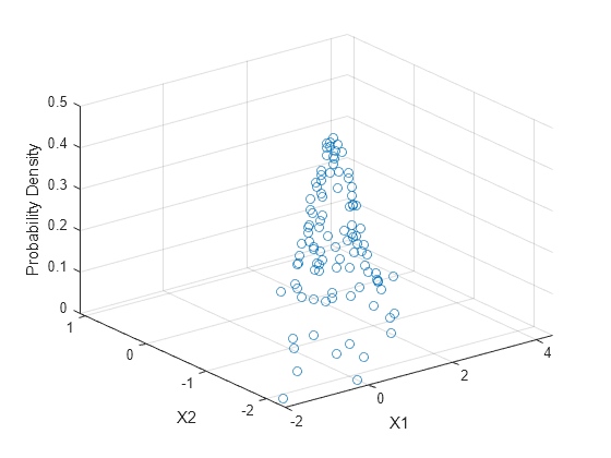
Plot the probability density values.

scatter3(X(:,1),X(:,2),y)
xlabel('X1')
ylabel('X2')
zlabel('Probability Density')

Multivariate Normal pdfs Evaluated at Same Point

Create ten different five-dimensional normal distributions, and compare the values of their pdfs at a specified point.

Set the dimensions n and d equal to 10 and 5, respectively.

n = 10;
d = 5;

Specify the means mu and the covariances Sigma of the multivariate normal distributions. Let all the distributions have the same mean vector, but vary the covariance matrices.

mu = ones(1,d)

mu = 1×5

     1     1     1     1     1

mat = eye(d);
nMat = repmat(mat,1,1,n);
var = reshape(1:n,1,1,n);
Sigma = nMat.*var;

Display the first two covariance matrices in Sigma.

Sigma(:,:,1:2)

ans = 
ans(:,:,1) =

     1     0     0     0     0
     0     1     0     0     0
     0     0     1     0     0
     0     0     0     1     0
     0     0     0     0     1


ans(:,:,2) =

     2     0     0     0     0
     0     2     0     0     0
     0     0     2     0     0
     0     0     0     2     0
     0     0     0     0     2

Set x to be a random point in five-dimensional space.

rng('default')  % For reproducibility
x = normrnd(0,1,1,5)

x = 1×5

    0.5377    1.8339   -2.2588    0.8622    0.3188

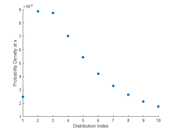
Evaluate the pdf at x for each of the ten distributions.

y = mvnpdf(x,mu,Sigma)

y = 10×1
10-4 ×

    0.2490
    0.8867
    0.8755
    0.7035
    0.5438
    0.4211
    0.3305
    0.2635
    0.2134
    0.1753

Plot the results.

scatter(1:n,y,'filled')
xlabel('Distribution Index')
ylabel('Probability Density at x')

Input Arguments

X — Evaluation points

numeric vector | numeric matrix

Evaluation points, specified as a 1-by-d numeric vector or an n-by-d numeric matrix, where n is a positive scalar integer and d is the dimension of a single multivariate normal distribution. The rows of X correspond to observations (or points), and the columns correspond to variables (or coordinates).

If X is a vector, then mvnpdf replicates it to match the leading dimension of mu or the trailing dimension of Sigma.

Data Types: single | double

mu — Means of multivariate normal distributions

vector of zeros (default) | numeric vector | numeric matrix

Means of multivariate normal distributions, specified as a 1-by-d numeric vector or an n-by-d numeric matrix.

• If mu is a vector, then mvnpdf replicates the vector to match the trailing dimension of Sigma.

• If mu is a matrix, then each row of mu is the mean vector of a single multivariate normal distribution.

Data Types: single | double

Sigma — Covariances of multivariate normal distributions

identity matrix (default) | symmetric, positive definite matrix | numeric array

Covariances of multivariate normal distributions, specified as a d-by-d symmetric, positive definite matrix or a d-by-d-by-n numeric array.

• If Sigma is a matrix, then mvnpdf replicates the matrix to match the number of rows in mu.

• If Sigma is an array, then each page of Sigma, Sigma(:,:,i), is the covariance matrix of a single multivariate normal distribution and, therefore, is a symmetric, positive definite matrix.

If the covariance matrices are diagonal, containing variances along the diagonal and zero covariances off it, then you can also specify Sigma as a 1-by-d vector or a 1-by-d-by-n array containing just the diagonal entries.

Data Types: single | double

Output Arguments

y — pdf values

numeric vector

pdf values, returned as an n-by-1 numeric vector, where n is one of the following:

• Number of rows in X if X is a matrix

• Number of times X is replicated if X is a vector

If X is a matrix, mu is a matrix, and Sigma is an array, then mvnpdf computes y(i) using X(i,:), mu(i,:), and Sigma(:,:,i).

More About

Multivariate Normal Distribution

The multivariate normal distribution is a generalization of the univariate normal distribution to two or more variables. It has two parameters, a mean vector μ and a covariance matrix Σ, that are analogous to the mean and variance parameters of a univariate normal distribution. The diagonal elements of Σ contain the variances for each variable, and the off-diagonal elements of Σ contain the covariances between variables.

The probability density function (pdf) of the d-dimensional multivariate normal distribution is

$$y\text{ = }f(x,\mu ,\Sigma )\text{ = }\frac{\text{1}}{\sqrt{\left|\Sigma \right|{\text{(2}\pi \text{)}}^d}}\exp \left(-\frac{\text{1}}{\text{2}}\text{(}x\text{-}\mu \text{) }{\Sigma }^{\text{-1}}\text{(}x\text{-}\mu \text{)'}\right)$$

where x and μ are 1-by-d vectors and Σ is a d-by-d symmetric, positive definite matrix. Only mvnrnd allows positive semi-definite Σ matrices, which can be singular. The pdf cannot have the same form when Σ is singular.

The multivariate normal cumulative distribution function (cdf) evaluated at x is the probability that a random vector v, distributed as multivariate normal, lies within the semi-infinite rectangle with upper limits defined by x:

$$\mathrm{Pr}\{v(1)\le x(1),v(2)\le x(2),\mathrm{...},v(d)\le x(d)\}.$$

Although the multivariate normal cdf does not have a closed form, mvncdf can compute cdf values numerically.

Tips

• In the one-dimensional case, Sigma is the variance, not the standard deviation. For example, mvnpdf(1,0,4) is the same as normpdf(1,0,2), where 4 is the variance and 2 is the standard deviation.

References

[1] Kotz, S., N. Balakrishnan, and N. L. Johnson. Continuous Multivariate Distributions: Volume 1: Models and Applications. 2nd ed. New York: John Wiley & Sons, Inc., 2000.

Extended Capabilities

C/C++ Code Generation
Generate C and C++ code using MATLAB® Coder™.

GPU Arrays

Accelerate code by running on a graphics processing unit (GPU) using Parallel Computing Toolbox™.

This function fully supports GPU arrays. For more information, see Run MATLAB Functions on a GPU (Parallel Computing Toolbox).

Version History

Introduced before R2006a