nlmefit
Fit nonlinear mixed-effects estimation
Syntax
Description
Examples
Load the sample data.
load orangetreedata.matThe vector c contains circumference measurements for five orange trees. The vector t contains the time at which the measurement was taken, and the vector id contains the tree id. The vector k contains the growth rate for each tree.
Create an anonymous function for the logistic growth equation.
model = @(phi,xfun,vfun)(phi(:,1))./(1+exp(-vfun(:).*(xfun-phi(:,2))));
model is a handle for a function given by the formula
.
The columns of the input argument phi correspond to the carrying capacity and midpoint for the logistic growth equation. xfun and vfun correspond to the time and logistic growth rate, respectively.
Fit model to the data in t, c, id, and k using the nlmefit function. Specify the initial estimate for each fixed-effect coefficient as 100.
beta = nlmefit(t,c,id,k,model,[100 100])
beta = 2×1

  129.6589
  121.4555
beta contains the fixed-effects estimates for the carrying capacity and midpoint.
Load the sample data.
load orangetreedata.matThe vector c contains circumference measurements for five orange trees. The vector t contains the time at which the measurement was taken, and the vector id contains the tree id. The vector k contains the growth rate for each tree.
Create an anonymous function for the logistic growth equation.
model = @(phi,xfun,vfun)(phi(:,1))./(1+exp(-vfun(:).*(xfun-phi(:,2))));
model is a handle for a function given by the formula
.
The columns of the input argument phi correspond to the carrying capacity and midpoint for the logistic growth equation. xfun and vfun correspond to the time and logistic growth rate, respectively.
Define an output function for nlmefit. For more information about the form of the output function, see the OutputFcn field description for the Options name-value argument.
function stop = outputFunction(beta,status,state)

    stop = 0;

    hold on
    plot3(status.iteration,beta(2),beta(1),"mo")

    state = string(state);

    if state=="done"
        stop=1;
    end

end
outputFunction plots the iteration number for the fitting algorithm together with the fixed effects. outputFunction returns 1 when the fitting algorithm completes its final iteration.
Use the statset function to create an options structure for nlmefit that uses outputFunction as its output function.
default_opts=statset("nlmefit");
opts = statset(default_opts,OutputFcn=@outputFunction);
opts is a statistics options structure that contains options for the fitting algorithm.
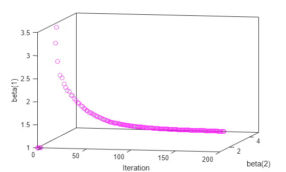
Create a figure and define axes in which to plot outputFunction. Fit model to the data in t, c, id, and k using the options in opts.
figure
ax = axes(view=[12,10]);
xlabel("Iteration")
ylabel("beta(2)")
zlabel("beta(1)")
box on

[beta,psi,stats] = nlmefit(t,c,id,k,model,[100 100],Options=opts)
beta = 2×1

  129.6589
  121.4555
psi = 2×2

  154.9857         0
         0    0.0000
stats = struct with fields:
           dfe: 30
          logl: -182.8139
           mse: 1.9029e+03
          rmse: 45.9892
    errorparam: 43.6225
           aic: 375.6279
           bic: 373.6750
          covb: [2×2 double]
        sebeta: [9.7010 2.7699]
          ires: [35×1 double]
          pres: [35×1 double]
         iwres: [35×1 double]
         pwres: [35×1 double]
         cwres: [35×1 double]
nlmefit calls outputFunction during the iterations of the fitting algorithm. The figure shows that the beta(1) and beta(2) fixed effects are near 126.5 and 129.6, respectively, when the iteration number is 0. The fitting algorithm calculates some estimates for beta(1) that are larger than 129.9 before converging to 129.66 in later iterations. Similarly, some estimates for beta(2) are larger than 122.2 in earlier iterations before converging to 121.5. The output argument beta contains the final values for the fixed effects. psi contains the covariance matrix for the random effects, and stats contains additional statistics about the fit.
Load the indomethacin data set.
load indomethacinThe variables time, concentration, and subject contain time series data for the blood concentration of the drug indomethacin in six patients.
Create an anonymous nonlinear function that accepts a vector of coefficients and a vector of predictor variables.
model = @(phi,t)(phi(1).*exp(-phi(2).*t)+phi(3).*exp(-phi(4).*t));
model is a handle for a function given by the formula
,
where is the concentration of indomethacin, for are coefficients, and is time. The function does not contain group-specific predictor variables because the formula does not include them.
Fit the model to the data using time as the predictor variable, subject as the grouping variable, and concentration as the response. Specify a log transformation function for the second and fourth coefficients.
phi0 = [1 1 1 1];
xform = [0 1 0 1];
[beta,psi,stats,b] = nlmefit(time,concentration, ...
   subject,[],model,phi0,ParamTransform=xform)
beta = 4×1
0.4606
-1.3459
2.8277
0.7729
psi = 4×4

    0.0124         0         0         0
         0    0.0000         0         0
         0         0    0.3264         0
         0         0         0    0.0250
stats = struct with fields:
           dfe: 57
          logl: 54.5882
           mse: 0.0066
          rmse: 0.0787
    errorparam: 0.0815
           aic: -91.1765
           bic: -93.0506
          covb: [4×4 double]
        sebeta: [0.1092 0.2244 0.2558 0.1066]
          ires: [66×1 double]
          pres: [66×1 double]
         iwres: [66×1 double]
         pwres: [66×1 double]
         cwres: [66×1 double]
b = 4×6

   -0.1111    0.0871    0.0670    0.0115   -0.1315    0.0769
         0         0         0         0         0         0
   -0.7396   -0.0704    0.8004   -0.5654    0.4127    0.1624
    0.0279    0.0287    0.0040   -0.2315    0.1984   -0.0276
The output argument beta contains the fixed effects for the model, and b contains the random effects. The maximum likelihood estimates for beta and the random-effects covariance matrix psi converge after about 300 iterations.
Plot the sample data together with the model, using only the fixed effects in beta for the model coefficients. Use the gscatter function to color code the data according to the subject. To reverse the log transformation on the second and fourth coefficients, take their exponentials using the exp function.
figure
hold on

gscatter(time,concentration,subject);

phi = [beta(1),exp(beta(2)),beta(3),exp(beta(4))];
tt = linspace(0,8);
cc = model(phi,tt);
plot(tt,cc,LineWidth=2,Color="k")

legend("Subject 1","Subject 2","Subject 3",...
    "Subject 4","Subject 5","Subject 6","Fitted curve")
xlabel("Time (hours)")
ylabel("Concentration (mcg/ml)")
title("Indomethacin Elimination")
hold off
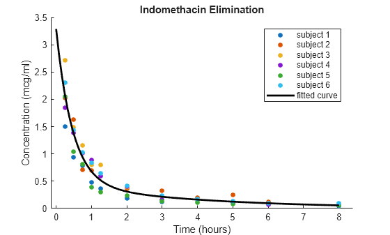
The plot shows that the blood concentration of indomethacin decreases over eight hours, and the fitted model passes through the bulk of the data.
Plot the data together with the model again, using both the fixed effects and the random effects in b for the model coefficients. For each subject, plot the data and the fitted curve in the same color.
figure
hold on

h = gscatter(time,concentration,subject);

for j=1:6
    phir = [beta(1)+b(1,j),exp(beta(2)+b(2,j)), ...
            beta(3)+b(3,j),exp(beta(4)+b(4,j))];
    ccr = model(phir,tt);
    col = h(j).Color;
    plot(tt,ccr,Color=col)
end

legend("Subject 1","Subject 2","Subject 3",...
    "Subject 4","Subject 5","Subject 6",...
    "Fitted curve 1","Fitted curve 2","Fitted curve 3",...
    "Fitted curve 4","Fitted curve 5","Fitted curve 6")
xlabel("Time (hours)")
ylabel("Concentration (mcg/ml)")
title("Indomethacin Elimination")

hold off

The plot shows that, for each subject, the fitted curve follows the bulk of the data more closely than the curve for the fixed-effects model in the previous figure. This result suggests that the random effects improve the fit of the model.
Input Arguments
Name-Value Arguments
Output Arguments
Algorithms
nlmefit fits the model by maximizing an estimate of the marginal
likelihood with the random effects removed by integration. During fitting, the function makes
the following assumptions:
The random effects come from a multivariate normal distribution and are independent between groups.
The observation errors come from the same normal distribution, and are independent of the random effects and each other. To change this default assumption, specify the
ErrorModelname-value argument.
References
[1] Lindstrom, M. J., and D. M. Bates. “Nonlinear Mixed-Effects Models for Repeated Measures Data.” Biometrics. Vol. 46, 1990, pp. 673–687.
[2] Davidian, M., and D. M. Giltinan. Nonlinear Models for Repeated Measurements Data. New York: Chapman & Hall, 1995.
[3] Pinheiro, J. C., and D. M. Bates. “Approximations to the Log-Likelihood Function in the Nonlinear Mixed-Effects MSodel.” Journal of Computational and Graphical Statistics. Vol. 4, 1995, pp. 12–35.
[4] Demidenko, E. Mixed Models: Theory and Applications. Hoboken, NJ: John Wiley & Sons, Inc., 2004.
Version History
Introduced in R2008b