plot
Plot receiver operating characteristic (ROC) curves and other performance curves
Since R2022a
Syntax
Description
plot( creates
a receiver operating characteristic (ROC) curve, which is a plot of the true positive
rate (TPR) versus the false positive rate (FPR), for each class in the rocObj)ClassNames property of the
rocmetrics object
rocObj. The function marks the model operating point for each
curve, and displays the value of the area under the ROC curve (AUC) and the class name for the curve in the legend.
plot(___, specifies
additional options using one or more name-value arguments in addition to any of the input
argument combinations in the previous syntaxes. For example,
Name=Value)AverageCurveType="macro",ClassNames=[] computes the average
performance metrics using the macro-averaging method and plots the average ROC curve
only.
[ also returns graphics objects for the model operating points and diagonal line.curveObj,graphicsObjs] = plot(___)
Examples
Create a rocmetrics object for a multiclass classification problem, and plot a ROC curve for each class.
Load the fisheriris data set. The matrix meas contains flower measurements for 150 different flowers. The vector species lists the species for each flower. species contains three distinct flower names.
load fisheririsTrain a classification tree that classifies observations into one of the three labels. Cross-validate the model using 10-fold cross-validation.
rng("default") % For reproducibility
Mdl = fitctree(meas,species,Crossval="on");
Compute the classification scores for validation-fold observations.
[~,Scores] = kfoldPredict(Mdl);
size(Scores)
ans = 1×2

   150     3
Scores is a matrix of size 150-by-3. The column order of Scores follows the class order in Mdl. Display the class order stored in Mdl.ClassNames.
Mdl.ClassNames
ans = 3×1 cell
    {'setosa'    }
    {'versicolor'}
    {'virginica' }
Create a rocmetrics object by using the true labels in species and the classification scores in Scores. Specify the column order of Scores using Mdl.ClassNames.
rocObj = rocmetrics(species,Scores,Mdl.ClassNames);
Plot the ROC curve for each class.
plot(rocObj)
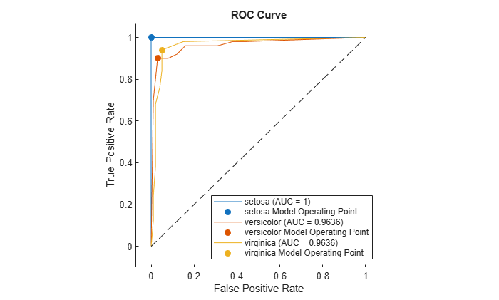
For each class, the plot function plots a ROC curve and displays a filled circle marker at the model operating point. The legend displays the class name and AUC value for each curve.
Plot the average ROC curve by using the plot function. Use a ROCCurve object, an output of the plot function, to obtain the average metric values.
Load the fisheriris data set. The matrix meas contains flower measurements for 150 different flowers. The vector species lists the species for each flower. species contains three distinct flower names.
load fisheririsTrain a classification tree that classifies observations into one of the three labels. Cross-validate the model using 10-fold cross-validation.
rng("default") % For reproducibility
Mdl = fitctree(meas,species,Crossval="on");
Compute the classification scores for validation-fold observations.
[~,Scores] = kfoldPredict(Mdl);
Create a rocmetrics object.
rocObj = rocmetrics(species,Scores,Mdl.ClassNames);
Plot the ROC curve for each class. Specify AverageCurveType="macro" to compute metrics for the average ROC curve using the macro-averaging method.
curveObj = plot(rocObj,AverageCurveType="macro")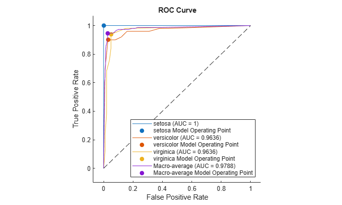
curveObj =
  4×1 ROCCurve array:

  ROCCurve    (setosa (AUC = 1))
  ROCCurve    (versicolor (AUC = 0.9636))
  ROCCurve    (virginica (AUC = 0.9636))
  ROCCurve    (Macro-average (AUC = 0.9788))
The plot function returns a ROCCurve object for each performance curve. You can use the object to query and set properties of the plot after creating it.
Display the data points of the average ROC curve stored in the fourth element of curveObj.
tbl_average = table(curveObj(4).Thresholds,curveObj(4).XData,curveObj(4).YData, ...
    VariableNames=["Threshold",curveObj(4).XAxisMetric,curveObj(4).YAxisMetric])
tbl_average=33×3 table
    Threshold    FalsePositiveRate    TruePositiveRate
    _________    _________________    ________________

           1                 0                  0
           1         0.0066667            0.60667
     0.95455              0.01               0.64
     0.95349              0.01               0.68
     0.95238          0.013333            0.72667
     0.95122          0.013333            0.82667
     0.91304          0.016667               0.86
     0.91111          0.023333            0.88667
     0.86957          0.026667            0.91333
         0.6          0.026667            0.92667
     0.33333          0.026667               0.94
         0.2          0.026667            0.94667
        -0.2              0.03            0.94667
    -0.33333          0.036667            0.94667
        -0.6          0.043333            0.94667
        -0.6          0.046667            0.94667
      ⋮
Create a rocmetrics object and plot performance curves by using the plot function. Specify the XAxisMetric and YAxisMetric name-value arguments of the plot function to plot different types of performance curves other than the ROC curve. If you specify new metrics when you call the plot function, the function computes the new metrics and then uses them to plot the curve.
Load the ionosphere data set. This data set has 34 predictors (X) and 351 binary responses (Y) for radar returns, either bad ('b') or good ('g').
load ionospherePartition the data into training and test sets. Use approximately 80% of the observations to train a support vector machine (SVM) model, and 20% of the observations to test the performance of the trained model on new data. Partition the data using cvpartition.
rng("default") % For reproducibility of the partition
c = cvpartition(Y,Holdout=0.20);
trainingIndices = training(c); % Indices for the training set
testIndices = test(c); % Indices for the test set
XTrain = X(trainingIndices,:);
YTrain = Y(trainingIndices);
XTest = X(testIndices,:);
YTest = Y(testIndices);
Train an SVM classification model.
Mdl = fitcsvm(XTrain,YTrain);
Compute the classification scores for the test set.
[~,Scores] = predict(Mdl,XTest);
Create a rocmetrics object. The rocmetrics function computes the FPR and TPR at different thresholds.
rocObj = rocmetrics(YTest,Scores,Mdl.ClassNames);
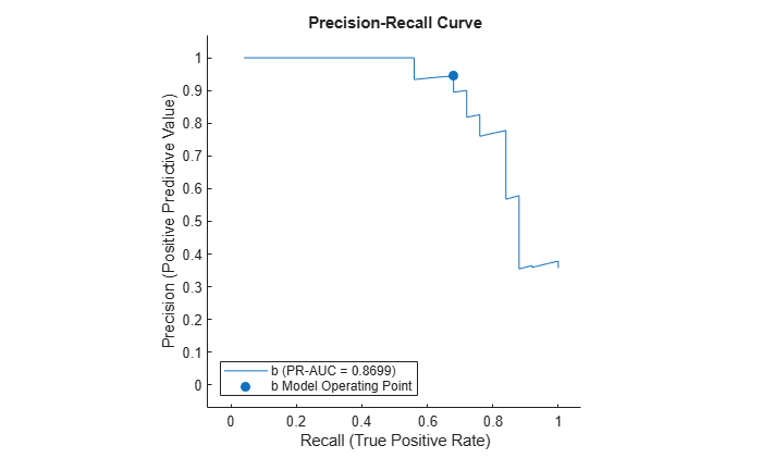
Plot the precision-recall curve for the first class. Specify the y-axis metric as precision (or positive predictive value) and the x-axis metric as recall (or true positive rate). The plot function computes the new metric values and plots the curve. Show the model operating point by setting the ShowModelOperatingPoint name-value argument to true.
curveObj = plot(rocObj,ClassNames=Mdl.ClassNames(1), ...
    YAxisMetric="PositivePredictiveValue",XAxisMetric="TruePositiveRate",...
    ShowModelOperatingPoint=true);
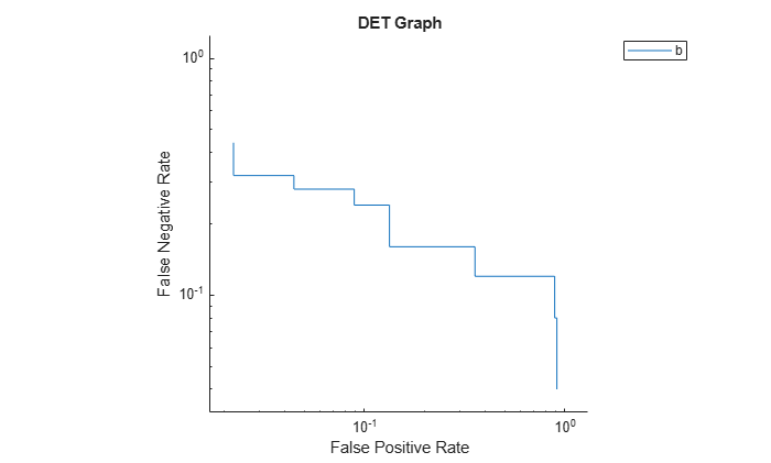
Plot the detection error tradeoff (DET) graph for the first class. Specify the y-axis metric as the false negative rate and the x-axis metric as the false positive rate. Use a log scale for the x-axis and y-axis.
f = figure;
plot(rocObj,ClassNames=Mdl.ClassNames(1), ...
    YAxisMetric="FalseNegativeRate",XAxisMetric="FalsePositiveRate")
f.CurrentAxes.XScale = "log";
f.CurrentAxes.YScale = "log";
title("DET Graph")
Compute the confidence intervals for FPR and TPR for fixed threshold values by using bootstrap samples, and plot the confidence intervals for TPR on the ROC curve.
Load the fisheriris data set. The matrix meas contains flower measurements for 150 different flowers. The vector species lists the species for each flower. species contains three distinct flower names.
load fisheririsTrain a naive Bayes model that classifies observations into one of the three labels. Cross-validate the model using 10-fold cross-validation.
rng("default") % For reproducibility
Mdl = fitcnb(meas,species,Crossval="on");
Compute the classification scores for validation-fold observations.
[~,Scores] = kfoldPredict(Mdl);
Create a rocmetrics object. Specify NumBootstraps as 100 to use 100 bootstrap samples to compute the confidence intervals.
rocObj = rocmetrics(species,Scores,Mdl.ClassNames, ...
    NumBootstraps=100);
Plot the ROC curve and the confidence intervals for TPR. Specify ShowConfidenceIntervals=true to show the confidence intervals.
plot(rocObj,ShowConfidenceIntervals=true)
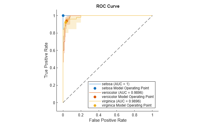
The shaded area around each curve indicates the confidence intervals. The widths of the confidence intervals for setosa are 0 for nonzero false positive rates, so the plot does not have a shaded area for setosa.
rocmetrics computes the ROC curves from the cross-validated scores. Therefore, each ROC curve represents an estimate of a ROC curve on unseen test data for a model trained on the full data set (meas and species). The confidence intervals represent the estimates of uncertainty for the curve. This uncertainty is due to the variance in unseen test data for the model trained on the full data set.
Compute the performance metrics (FPR and TPR) for a binary classification problem by creating a rocmetrics object, and plot a ROC curve by using the plot function. The plot function displays a filled circle at the model operating point. Display a data tip at the model operating point.
Load the ionosphere data set. This data set has 34 predictors (X) and 351 binary responses (Y) for radar returns, either bad ('b') or good ('g').
load ionospherePartition the data into training and test sets. Use approximately 80% of the observations to train a support vector machine (SVM) model, and 20% of the observations to test the performance of the trained model on new data. Partition the data using cvpartition.
rng("default") % For reproducibility of the partition
c = cvpartition(Y,Holdout=0.20);
trainingIndices = training(c); % Indices for the training set
testIndices = test(c); % Indices for the test set
XTrain = X(trainingIndices,:);
YTrain = Y(trainingIndices);
XTest = X(testIndices,:);
YTest = Y(testIndices);
Train an SVM classification model.
Mdl = fitcsvm(XTrain,YTrain);
Compute the classification scores for the test set.
[~,Scores] = predict(Mdl,XTest);
Create a rocmetrics object.
rocObj = rocmetrics(YTest,Scores,Mdl.ClassNames);
The rocmetrics function computes the FPR and TPR at different thresholds and finds the AUC value.
Plot the ROC curve. Specify ClassNames to plot the curve for the first class.
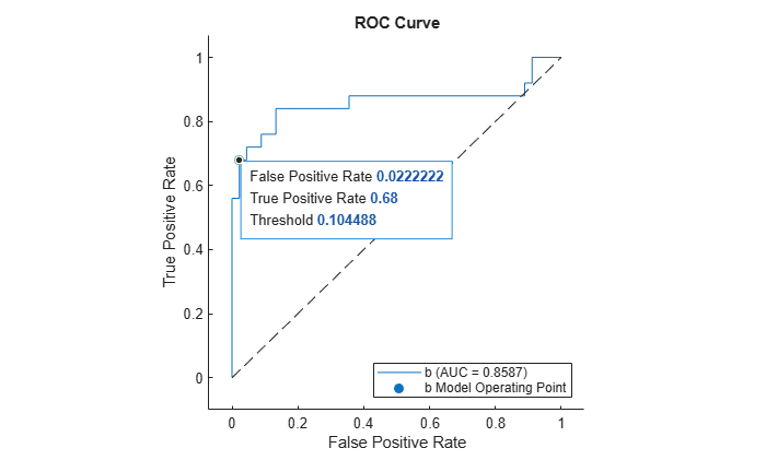
curveObj = plot(rocObj,ClassNames=Mdl.ClassNames(1));
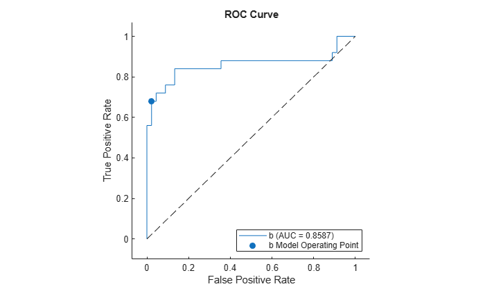
The plot function returns a ROCCurve object for each performance curve. You can use the object to query and set the properties of the plot after creating it.
The filled circle marker indicates the model operating point at which the threshold value is 0. The function chooses a point that has the largest threshold value less than or equal to 0. The legend displays the class name and AUC value for the curve.
You can create data tips by clicking data points on the curve. Alternatively, you can create data tips using the datatip function.
Find the model operating point in the Metrics property of rocObj for class b. The predict function classifies an observation into the class yielding a larger score, which corresponds to the class with a nonnegative adjusted score. That is, the typical threshold value used by the predict function is 0. Among the rows in the Metrics property of rocObj for class b, find the point that has the smallest nonnegative threshold value. The point on the curve indicates identical performance to the performance of the threshold value 0.
idx_b = strcmp(rocObj.Metrics.ClassName,"b");
t = rocObj.Metrics(idx_b,:);
X = rocObj.Metrics(idx_b,:).FalsePositiveRate;
Y = rocObj.Metrics(idx_b,:).TruePositiveRate;
T = rocObj.Metrics(idx_b,:).Threshold;
idx_model = find(T>=0,1,"last");
modelpt = [T(idx_model) X(idx_model) Y(idx_model)]
modelpt = 1×3

    0.1045    0.0222    0.6800
Display a data tip at the model operating point. Specify the target graph object as the output object of the plot function.
datatip(curveObj,DataIndex=idx_model,Location="southeast");