Analyze Transfer Function of T-Coil Circuit

This example shows how to analyze the transfer function of a T-coil circuit using Symbolic Math Toolbox™ and Control System Toolbox™. In this example, you define symbolic equations, solve for the transfer function, and analyze the stability, frequency response, and step response of the circuit.

The T-coil (or bridged T-coil) is a circuit topology that extends the signal bandwidth by a greater factor than inductive peaking does. The T-coil consists of two mutually coupled inductors and a bridge capacitor. This figure illustrates the T-coil circuit that you analyze in this example.

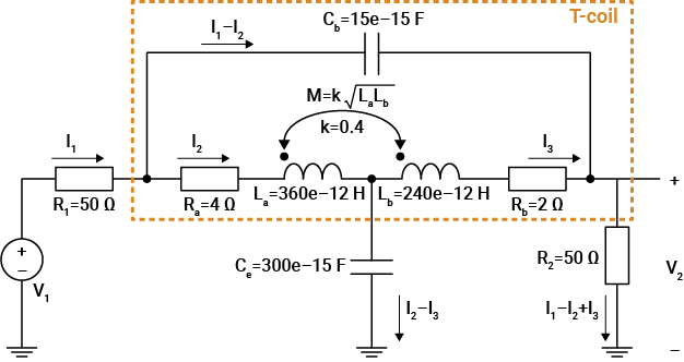
These variables describe the circuit:

• V1 is the input voltage.

• V2 is the output voltage.

• I1, I2, and I3 are the currents that flow on specific paths of the circuit.

• R1 is the resistor connected to the input voltage.

• R2 is the resistor connected to the output voltage.

• Ra is the parasitic resistance of the inductor La.

• Rb is the parasitic resistance of the inductor Lb.

• La is the first inductor in the T-coil.

• Lb is the second inductor in the T-coil.

• M is the mutual inductance between the inductors La and Lb, where k is the coefficient of coupling.

• Cb is the bridge capacitor in the T-coil.

• Ce is the capacitor that connects one of the T-coil terminals to the ground.

Define Symbolic Variables and Equations

Define the symbolic variables for voltages, currents, resistances, inductances, mutual inductance, and capacitances. Additionally, define the Laplace variable s, which represents the complex frequency that describes the circuit in the Laplace domain.

syms V1 V2 I1 I2 I3
syms R1 R2 Ra Rb La Lb M Cb Ce s

Create a system of equations that represents the T-coil circuit. Apply Kirchhoff's voltage and current laws in the Laplace domain to obtain the system of equations.

eqn1 = V1 == R1*I1 + 1/(Cb*s)*(I1-I2) + V2;
eqn2 = V1 == R1*I1 + Ra*I2 + M*s*I3 + La*s*I2 + 1/(Ce*s)*(I2-I3);
eqn3 = V2 == R2*(I1-I2+I3);
eqn4 = V2 == -Rb*I3 - M*s*I2 - Lb*s*I3 + 1/(Ce*s)*(I2-I3);
eqns = [eqn1; eqn2; eqn3; eqn4]

eqns = 
$$\left(\begin{array}{c}{V}_1=V_2+I_1\hspace{0.17em}{R}_1+\frac{I_1-I_2}{\mathrm{Cb}\hspace{0.17em}s}\\ V_1=I_1\hspace{0.17em}{R}_1+I_2\hspace{0.17em}\mathrm{Ra}+\frac{I_2-I_3}{\mathrm{Ce}\hspace{0.17em}s}+I_2\hspace{0.17em}\mathrm{La}\hspace{0.17em}s+I_3\hspace{0.17em}M\hspace{0.17em}s\\ V_2=R_2\hspace{0.17em}\left(I_1-I_2+I_3\right)\\ V_2=\frac{I_2-I_3}{\mathrm{Ce}\hspace{0.17em}s}-I_3\hspace{0.17em}\mathrm{Rb}-I_3\hspace{0.17em}\mathrm{Lb}\hspace{0.17em}s-I_2\hspace{0.17em}M\hspace{0.17em}s\end{array}\right)$$

Analyze Transfer Function of Input Voltage to Output Voltage

The system of equations consists of four linearly independent equations, so you can solve for four unknowns from the equations. For this reason, explicitly specify the four variables you want to solve for when using solve. Solve the system of equations for the variables I1, I2, V1, and V2. The solve function returns the solutions as a structure in result.

result = solve(eqns,I1,I2,V1,V2);

Next, find the transfer function by calculating the ratio of the output voltage to the input voltage.

V2_over_V1 = result.V2/result.V1;

Define numerical values for the circuit parameters in SI units.

params.R1 = 50;
params.R2 = 50;
params.Ra = 4;
params.Rb = 2;
params.La = 360e-12;
params.Lb = 240e-12;
params.M  = 0.4*sqrt(params.La*params.Lb);
params.Cb = 15e-15;
params.Ce = 300e-15;

Substitute the values for the circuit parameters into the transfer function. Use vpa to compute the transfer function to five digits of accuracy. Here, the transfer function is in symbolic form.

h_tcoil = vpa(subs(V2_over_V1,params),5)

h_tcoil = 
$$\frac{50.0\hspace{0.17em}\left(3.2659e-46\hspace{0.17em}{s}^4+7.56e-36\hspace{0.17em}{s}^3-2.2709e-23\hspace{0.17em}{s}^2+9.0e-14\hspace{0.17em}s+1.0\right)}{3.2659e-44\hspace{0.17em}{s}^4+3.1924e-32\hspace{0.17em}{s}^3+1.0828e-20\hspace{0.17em}{s}^2+1.6866e-9\hspace{0.17em}s+106.0}$$

To convert the transfer function to a numeric form, first extract the numerator and denominator of the transfer function by using numden.

[n,d] = numden(h_tcoil);

Convert the numerator and denominator to numeric vectors of polynomial coefficients by using sym2poly. Based on these coefficients, construct the transfer function model using Control System Toolbox. Use minreal to eliminate the uncontrollable state of the transfer function, or in other words, to cancel the pole-zero pairs in the transfer function.

h_tcoil = tf(sym2poly(n),sym2poly(d));
h_tcoil = minreal(h_tcoil)

h_tcoil =
 
  0.5 s^4 + 1.157e10 s^3 - 3.477e22 s^2 + 1.378e32 s + 1.531e45
  -------------------------------------------------------------
    s^4 + 9.775e11 s^3 + 3.315e23 s^2 + 5.164e34 s + 3.246e45
 
Continuous-time transfer function.
Model Properties

Pole-Zero Map

Plot the pole-zero map of the transfer function by using pzmap. This system has four complex zeros, marked by o on the plot. The system also has a pair of complex poles and two real poles, marked by x.

figure(1)
pzmap(h_tcoil)

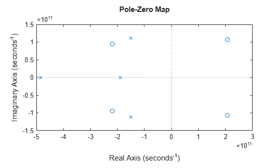
To obtain the values of these poles and zeros, use pzmap with two output arguments.

[p,z] = pzmap(h_tcoil)

p = 4×1 complex
1011 ×

  -4.8499 + 0.0000i
  -1.9025 + 0.0000i
  -1.5113 + 1.1107i
  -1.5113 - 1.1107i

z = 4×1 complex
1011 ×

   2.0656 + 1.0722i
   2.0656 - 1.0722i
  -2.1813 + 0.9460i
  -2.1813 - 0.9460i

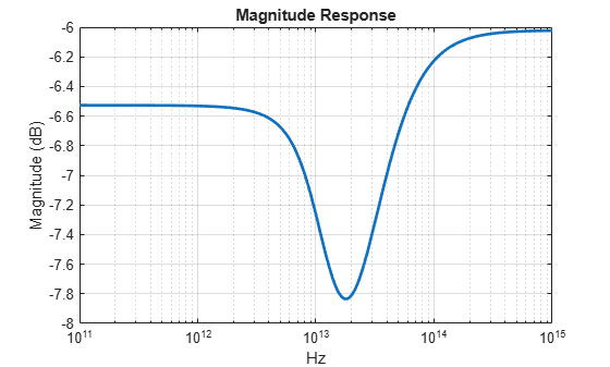
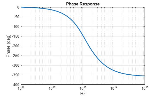
Bode Plot

Create a Bode plot of the frequency response of the transfer function. The plot displays the magnitude (in dB) and phase (in degrees) of the system response as a function of frequency.

To obtain the values of the magnitude and the phase of the system response at specific frequencies, use the bode function with three output arguments. Because bode uses radians per second (rad/s) as the frequency units, define the frequencies where you want to compute the magnitude and phase in rad/s.

w = linspace(1e11,1e15,4000)*pi/180;
[mag,phz,w] = bode(h_tcoil,w);

Convert the output frequencies from rad/s to Hz.

f = w*180/pi;

Convert the magnitude from absolute units to decibels.

magdb = 20*log10(mag(:));

Next, plot the magnitude response by using semilogx.

figure(2)
semilogx(f,magdb,LineWidth=2)
grid on
xlabel("Hz")
ylabel("Magnitude (dB)")
title("Magnitude Response")

Then, ensure the phase response is 0 degrees at low frequencies (DC) instead of a multiple of 360 degrees. Introducing an offset, phz(1), to the phase response vector does not change the effective phase response, but it makes the plot more intuitive.

phz = phz(:) - phz(1);
figure(3)
semilogx(f,phz,LineWidth=2)
grid on
xlabel("Hz")
ylabel("Phase (deg)")
title("Phase Response")

Step Response

Plot the step response of the transfer function by using step.

figure(4)
step(h_tcoil)
grid on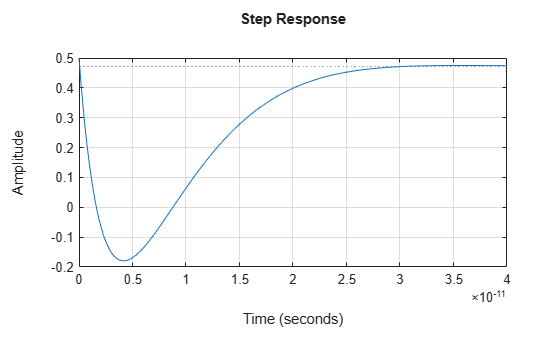

Compare Transfer Functions with and without Parasitic Resistances

In the previous sections, the parasitic resistances of the two inductors are assumed to be 4 ohms and 2 ohms. To compare the transfer function responses for an ideal case where the parasitic resistances are zero, you can repeat a similar process but substitute the values of Ra and Rb with 0 ohms.

params.Ra = 0;
params.Rb = 0;

Find the transfer function without parasitic resistances.

h_tcoil_ideal = vpa(subs(V2_over_V1,params),5)

h_tcoil_ideal = 
$$\frac{50.0\hspace{0.17em}\left(3.2659e-46\hspace{0.17em}{s}^4-2.2745e-23\hspace{0.17em}{s}^2+1.0\right)}{3.2659e-44\hspace{0.17em}{s}^4+3.1168e-32\hspace{0.17em}{s}^3+1.0253e-20\hspace{0.17em}{s}^2+1.5852e-9\hspace{0.17em}s+100.0}$$

[n,d] = numden(h_tcoil_ideal);
h_tcoil_ideal = tf(sym2poly(n),sym2poly(d));
h_tcoil_ideal = minreal(h_tcoil_ideal)

h_tcoil_ideal =
 
  0.5 s^4 + 0.0003357 s^3 - 3.482e22 s^2 - 1.729e19 s + 1.531e45
  --------------------------------------------------------------
    s^4 + 9.543e11 s^3 + 3.139e23 s^2 + 4.854e34 s + 3.062e45
 
Continuous-time transfer function.
Model Properties

Next, plot the magnitude response of the transfer function without parasitic resistances.

[mag_ideal,phz_ideal,w] = bode(h_tcoil_ideal,w);
f = w*180/pi;
magdb_ideal = 20*log10(mag_ideal(:));
figure(2)
hold on
semilogx(f,magdb_ideal,"r:",LineWidth=2)
legend("With parasitics","Without parasitics")

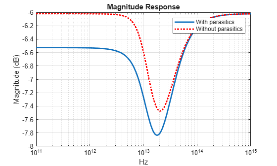
Here, you can see that the maximum attenuation of the T-coil occurs at a frequency of 2.1e13 Hz for the case without parasitic resistances, compared to a frequency of 1.78e13 Hz for the case with parasitic resistances. Additionally, for the case without parasitic resistances, the magnitude response at low and high frequencies is around –6 dB. Meanwhile, for the case with parasitic resistances, the magnitude response at low frequencies is around –6.53 dB.

Then, plot the phase response of the transfer function without parasitic resistances by introducing an offset to make the phase response equal to 0 at the minimum frequency range.

phz_ideal = phz_ideal(:) - phz_ideal(1);
figure(3)
hold on
semilogx(f,phz_ideal,"r:",LineWidth=2)
legend("With parasitics","Without parasitics")

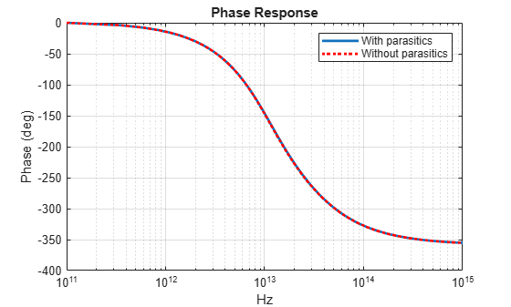
The phase responses for the cases with and without parasitic resistances are very close to each other, within 1 degree.

Analyze Transfer Function of Input Current to Output Voltage

Suppose you want to analyze the transfer function for the ratio of the output voltage V2 to the input current I1 (the transimpedance transfer function). You can compute this transfer function from the solutions of V2 and I1 that you obtained in the previous section. Calculate the ratio of result.V2 to result.I1, and simplify the result. Using a similar process as in the previous sections, you can then analyze this transfer function using Control System Toolbox.

V2_over_I1 = simplify(result.V2/result.I1);
params.Ra = 4;
params.Rb = 2;
z_tcoil = vpa(subs(V2_over_I1,params),5)

z_tcoil = 
$$\frac{50.0\hspace{0.17em}\left(3.2659e-46\hspace{0.17em}{s}^4+7.56e-36\hspace{0.17em}{s}^3-2.2709e-23\hspace{0.17em}{s}^2+9.0e-14\hspace{0.17em}s+1.0\right)}{3.2659e-46\hspace{0.17em}{s}^4+1.9547e-34\hspace{0.17em}{s}^3+8.5913e-23\hspace{0.17em}{s}^2+1.569e-11\hspace{0.17em}s+1.0}$$

[n,d] = numden(z_tcoil);
z_tcoil = tf(sym2poly(n),sym2poly(d));
z_tcoil = minreal(z_tcoil)

z_tcoil =
 
  50 s^4 + 1.157e12 s^3 - 3.477e24 s^2 + 1.378e34 s + 1.531e47
  ------------------------------------------------------------
   s^4 + 5.985e11 s^3 + 2.631e23 s^2 + 4.804e34 s + 3.062e45
 
Continuous-time transfer function.
Model Properties

References

[1] Razavi, Behzad. "The Bridged T-Coil [A Circuit for All Seasons]." IEEE Solid-State Circuits Magazine 7, no. 4 (Fall 2015): 9–13. https://doi.org/10.1109/MSSC.2015.2474258.

[2] Kossel, Marcel, Christian Menolfi, Jonas Weiss, Peter Buchmann, George von Bueren, Lucio Rodoni, Thomas Morf, Thomas Toifl, and Martin Schmatz. "A T-Coil-Enhanced 8.5Gb/s High-Swing Source-Series-Terminated Transmitter in 65nm Bulk CMOS." In 2008 IEEE International Solid-State Circuits Conference - Digest of Technical Papers, 110–599. San Francisco, CA, USA: IEEE 2008. https://doi.org/10.1109/ISSCC.2008.4523081.