Visualize PX4 Hardware-in-the-Loop (HITL) Simulation with UAV Dynamics in Simulink

R2026b

This example shows how to simulate UAV dynamics and visualize PX4® Hardware-in-the-Loop (HITL) simulation. You can visualize the simulation using either 3D Scenarios or Unreal Engine®.

Example Requirements

Prerequisites

1. For an introduction to Simulink, watch the Simulink Quick Start video.

2. Configure and set up Pixhawk in HITL mode. For more information, see Setting Up PX4 Autopilot in Hardware-in-the-Loop (HITL) Mode from QGroundControl.

3. Set up the PX4 firmware as described in Set Up PX4 Firmware for Hardware-in-the-Loop (HITL) Simulation. In the Select a PX4 Autopilot and Build Target screen, select any Pixhawk Series board. Then select the corresponding build target that contains the _multicopter keyword. This example uses Pixhawk 6x with the px4_fmu-v6x_multicopter build target.

4. Open two instances of MATLAB®:

   1. First instance — Deploy the flight controller and run the UAV dynamics model.

   2. Second instance — Run the visualization.

Required Hardware

• Pixhawk® Series flight controller (this example uses Pixhawk 6x), connected to the host computer using the USB cable.

• Micro USB type-B cable.

• Micro-SD card.

This diagram shows the HITL setup and physical connections between modules.

Required Software

This example requires QGroundControl.

Open Project in First Instance of MATLAB

Launch the first instance of MATLAB. To access the Simulink model, supporting files, and project shortcuts that this example uses, open the PX4demo_HITLSimulinkPlant.prj project file.

prj = openProject("PX4demo_HITLSimulinkPlant");

Copy the current folder path to the clipboard. You use this path later to open the project in the second MATLAB instance.

clipboard("copy",pwd)

Deploy Autopilot Controller Model to Pixhawk Board in First Instance of MATLAB

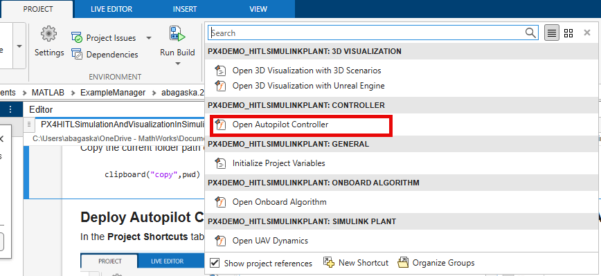
To launch the controller model, on the Project tab, click Open Autopilot Controller.

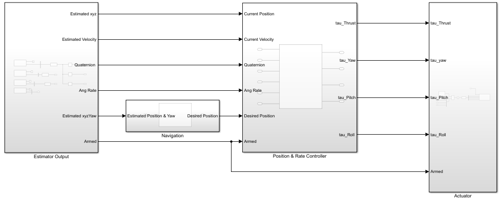
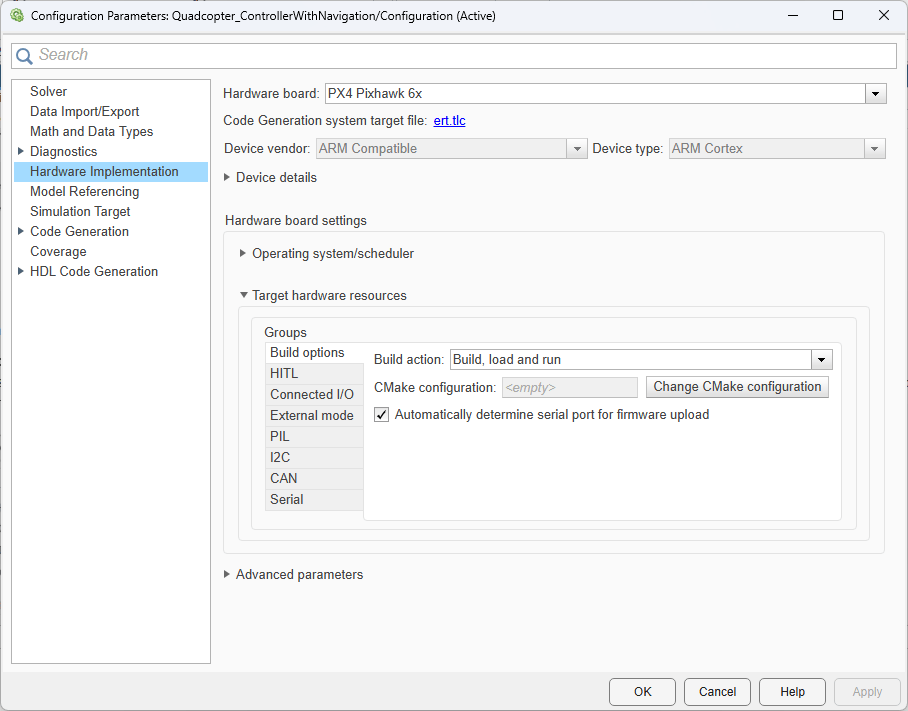
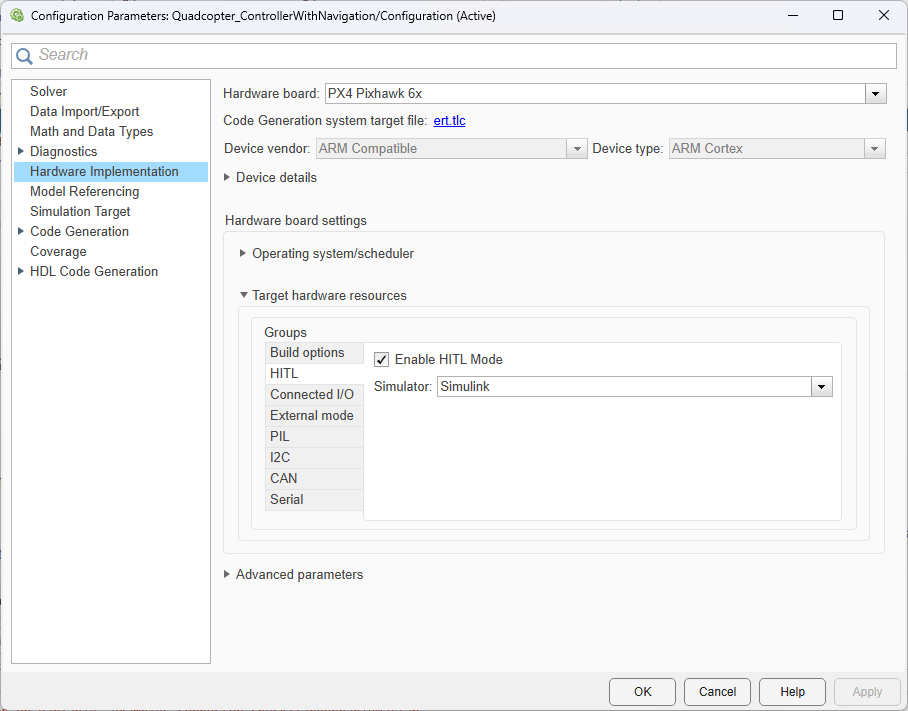
On the Simulink Toolstrip, on the Hardware tab, click Hardware Settings. In the left pane, select Hardware Implementations, and verify these options:

• Verify that Hardware board is set to PX4 Pixhawk 6x (or your Pixhawk board).

• In the Hardware board settings section, under Target hardware resources, select the Build options tab of the Groups pane. Verify that Build action is set to Build, load and run.

• Select the HITL tab of the Groups pane. Verify that Simulator is set to Simulink and Enable HITL Mode is selected.

After you verify the settings, on the Simulink Toolstrip, on the Hardware tab, in the Deploy section, click Build, Deploy & Start.

Simulink generates and deploys code to the Pixhawk board. After deployment completes, QGroundControl opens automatically.

Run UAV Dynamics Model in First Instance of MATLAB

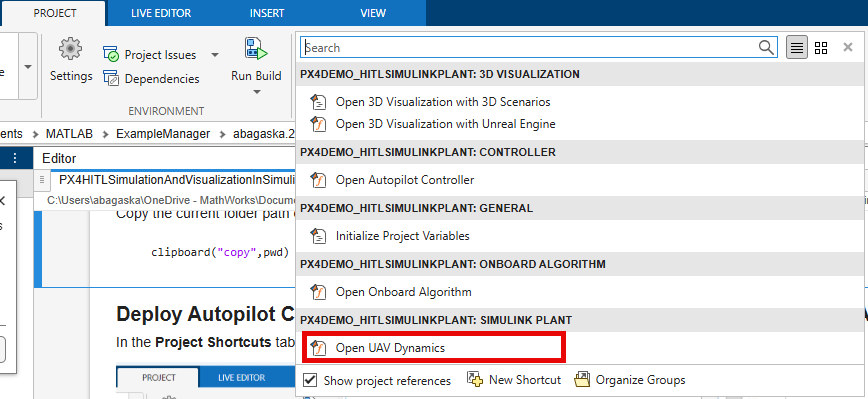
To launch the plant model, on the Project tab, click Open UAV Dynamics.

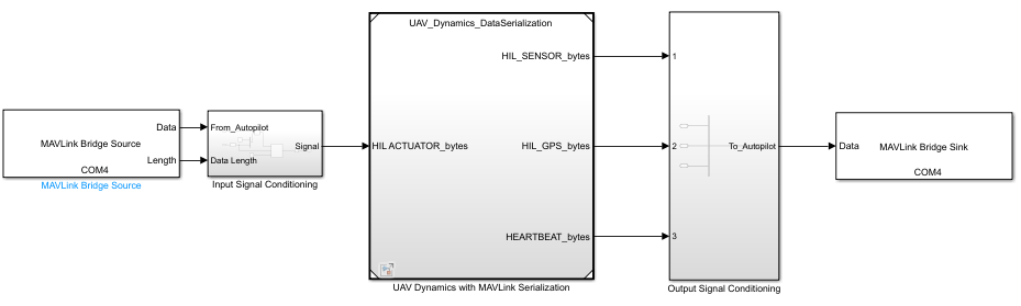
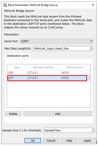
To configure the connection for flight visualization, open the MAVLink Bridge Source block. Verify that the block receives MAVLink data from the PX4 Autopilot over UDP port 25000.

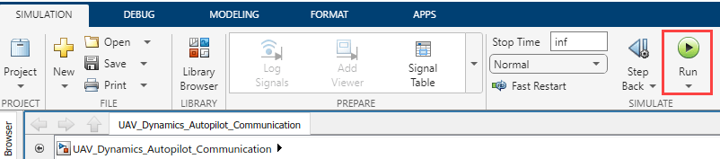
To simulate the model, on the Simulink Toolstrip of the plant model, on the Simulation tab, click Run.

Set Reference Location of Plant Model in First Instance of MATLAB

The provided predefinedMission.plan file is configured for the Natick, MA location. To match this location, set the GPS reference point and magnetic field in the UAV Dynamics model. Run these commands in the MATLAB Command Window.

ref_lat = 42.2990986;          % Latitude [deg] (Natick, MA)
ref_lon = -71.3504025;         % Longitude [deg] (Natick, MA)
ref_height = 50;               % Altitude [m]
magNED = [20.04 -4.94 46.84];  % Magnetic field in NED frame [microtesla]

The model now uses the Natick, MA reference location.

Create and Start Mission in QGroundControl

Open QGroundControl, and then configure and assign the actuators of the quadcopter. For more details, see Configure and Assign Actuators in QGroundControl.

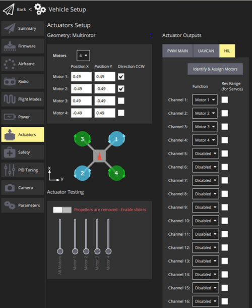
To load and upload the mission plan:

1. At the top of the QGroundControl interface, next to Connected, click the QGroundControl logo and select Plan Flight.

2. Load the predefinedMission.plan file from the data folder of the project directory.

3. Click Upload Required. Then, click Upload.

4. To return to the Fly View, click Exit Plan.

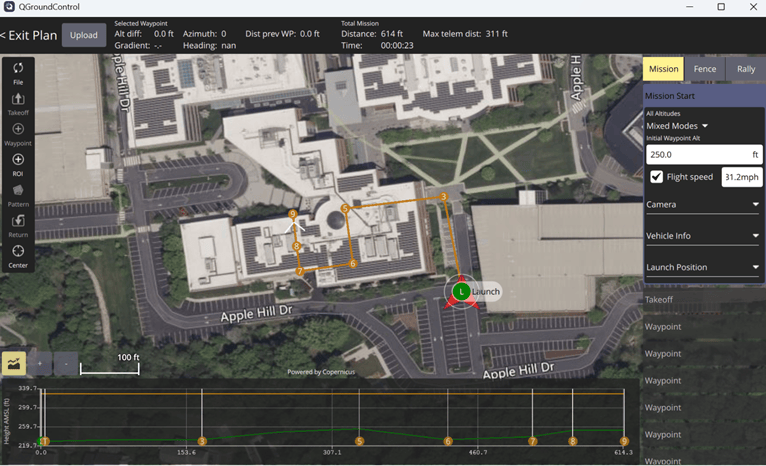
You can also create your own mission and upload it. By default, the UAV Dynamics model supports only these types of mission commands:

• Takeoff

• Land

• Waypoint

Open Project in Second Instance of MATLAB

Launch a second instance of MATLAB. Right-click the address bar and select Paste and Go to navigate to the folder path you copied from the first MATLAB instance.

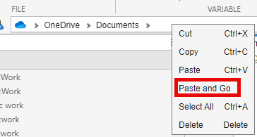
To access the Simulink model, supporting files, and project shortcuts that this example uses, open the PX4demo_HITLSimulinkPlant.prj project file.

prj = openProject("PX4demo_HITLSimulinkPlant");

Before starting the mission, verify that QGroundControl displays Ready To Fly. Then, follow the steps for your preferred visualization method: 3D Scenarios (Option 1) or Unreal Engine (Option 2).

Option 1: Visualize with 3D Scenarios in Second Instance of MATLAB

To launch the 3D Scenario viewer, on the Project tab, click Open 3D Visualization with 3D Scenarios.

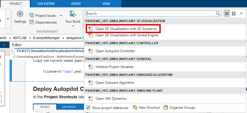
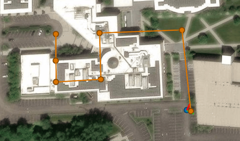
The 3D Scenario viewer automatically displays the predefined mission path.

In the Fly View of QGroundControl, start the mission by using the slider or holding the spacebar.

The UAV follows the mission path, and the flight is shown in 3D Scenarios.

To properly close the 3D Scenario viewer after the simulation completes, disconnect the receiver.

clear handleMAVLink
disconnect(receiver);

Option 2: Visualize with Unreal Engine in Second Instance of MATLAB

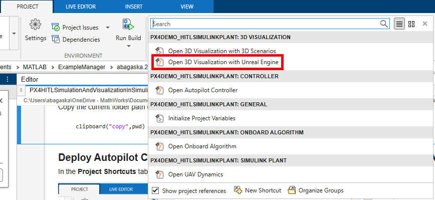
To launch the Unreal visualization model, on the Project tab, click Open 3D Visualization with Unreal Engine.

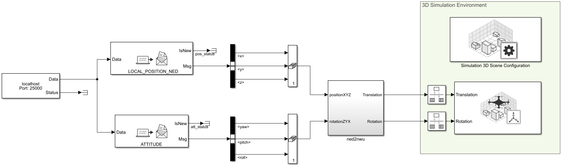
This model receives MAVLink data from the PX4 Autopilot over UDP port 25000, decodes UAV position and attitude, and converts coordinates for 3D visualization. The MAVLink Bridge Source block handles reception and decoding, and the Simulation 3D UAV Vehicle block renders the flight.

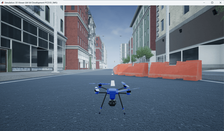
To simulate the model, on the Simulation tab, click Run. After the model starts, the Unreal Engine simulation environment opens.

In the Fly View of QGroundControl, start the mission by using the slider or holding the spacebar.

The UAV follows the mission path, and the flight is shown in Unreal Engine.

Troubleshooting

• If you see the error some modules could not be found while simulating the visualization model, change the compiler to Microsoft Visual C++ 2019 by running mex --setup C++.

• If the Unreal Engine simulation is slow, check that your host PC has a GPU with a compute capability of 5.0 or higher.