Examples Using Wavelet Packet Tree Objects
You can use command line functions to work with wavelet packet trees (WPTREE objects). The most useful commands are:
We can see some of these features in the following examples.
plot and wpviewcf
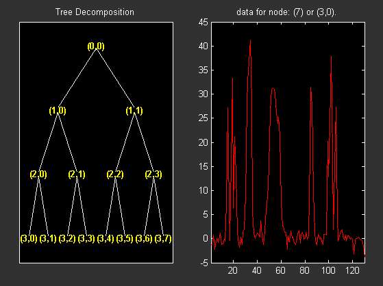
load noisbump
x = noisbump;
t = wpdec(x,3,'db2');
fig = plot(t);
Click on node 7.
Change Node Action from Visualize to Split-Merge and merge the second node.
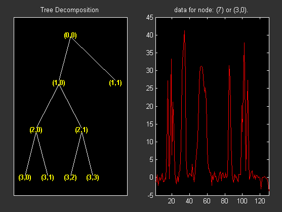
% From the command line, you can get the new tree.
newt = plot(t,'read',fig);

% The first argument of the plot function in the last command
% is dummy. Then the general syntax is:
%    newt = plot(DUMMY,'read',fig);
% where DUMMY is any object parented by an NTREE object.
% DUMMY can be any object constructor name, which returns
% an object parented by an NTREE object. For example:
%    newt = plot(ntree,'read',fig);
%    newt = plot(dtree,'read',fig);
%    newt = plot(wptree,'read',fig);

% From the command line you can modify the new tree,
% then plot it.
newt = wpjoin(newt,3);
fig2 = plot(newt);

% Change Node Label from Depth_position to Index and
% click the node (3). You get the following figure.
% Using plot(newt,fig), the plot is done in the figure fig,
% which already contains a tree object.

% You can see the colored wavelet packets coefficients using
% from the command line, the wpviewcf function (type help
% wpviewcf for more information).
wpviewcf(newt,1)

% You get the following plot, which contains the terminal nodes
% colored coefficients.
Change Terminal Node Coefficients
load gatlin2
t = wpdec2(X,1,'haar');
plot(t);
% Change Node Label from Depth_position to Index and
% click the node (0). You get the following figure.
% Now modify the coefficients of the four terminal nodes.
newt = t;
NBcols = 40;

for node = 1:4
  cfs = read(t,'data',node);
  tmp = cfs(1:end,1:NBcols);
  cfs(1:end,1:NBcols) = cfs(1:end,end-NBcols+1:end);
  cfs(1:end,end-NBcols+1:end) = tmp;
  newt = write(newt,'data',node,cfs);
end
plot(newt)

% Change Node Label from Depth_position to Index and
% click on the node (0). You get the following figure.
You can use this method for a more useful purpose. Let's see a denoising example.
Thresholding Wavelet Packets
load noisbloc
x = noisbloc;
t = wpdec(x,3,'sym4');
plot(t);
% Change Node Label from Depth_position to Index and
% click the node (0). You get the following plot.
% Global thresholding.
t1 = t;
sorh = 'h';
thr = wthrmngr('wp1ddenoGBL','penalhi',t);
cfs = read(t,'data');
cfs = wthresh(cfs,sorh,thr);
t1  = write(t1,'data',cfs);
plot(t1)

% Change Node Label from Depth_position to Index and
% click the node (0). You get the following plot.
% Node by node thresholding.
t2 = t;
sorh = 's';
thr(1) = wthrmngr('wp1ddenoGBL','penalhi',t);
thr(2) = wthrmngr('wp1ddenoGBL','sqtwologswn',t);
tn  = leaves(t);
for k=1:length(tn)
  node = tn(k);
  cfs = read(t,'data',node);
  numthr = rem(node,2)+1;
  cfs = wthresh(cfs,sorh,thr(numthr));
  t2 = write(t2,'data',node,cfs);
end
plot(t2)

% Change Node Label from Depth_position to Index and
% click the node (0). You get the following plot.