Spoken Digit Recognition with Wavelet Scattering and Deep Learning
This example shows how to classify spoken digits using both machine and deep learning techniques. In the example, you perform classification using wavelet time scattering with a support vector machine (SVM) and with a long short-term memory (LSTM) network. You also apply Bayesian optimization to determine suitable hyperparameters to improve the accuracy of the LSTM network. In addition, the example illustrates an approach using a deep convolutional neural network (CNN) and mel-frequency spectrograms.
Data
Download the Free Spoken Digit Dataset (FSDD) [1]. FSDD consists of 2000 recordings in English of the digits 0 through 9 obtained from four speakers. Two of the speakers are native speakers of American English, one speaker is a nonnative speaker of English with a Belgian French accent, and one speaker is a nonnative speaker of English with a German accent. The data is sampled at 8000 Hz.
downloadFolder = matlab.internal.examples.downloadSupportFile("audio","FSDD.zip");
dataFolder = tempdir;
unzip(downloadFolder,dataFolder)
dataset = fullfile(dataFolder,"FSDD");
Use audioDatastore (Audio Toolbox) to manage data access and ensure the random division of the recordings into training and test sets. Create an audioDatastore that points to the dataset.
ads = audioDatastore(dataset,IncludeSubfolders=true);
The helper function helpergenLabels creates a categorical array of labels from the FSDD files. The source code for helpergenLabels is listed in the appendix. List the classes and the number of examples in each class.
ads.Labels = helpergenLabels(ads);
summary(ads.Labels)
2000×1 categorical

     0                200
     1                200
     2                200
     3                200
     4                200
     5                200
     6                200
     7                200
     8                200
     9                200
     <undefined>        0
The FSDD data set consists of 10 balanced classes with 200 recordings each. The recordings in the FSDD are not of equal duration. The FSDD is not prohibitively large, so read through the FSDD files and construct a histogram of the signal lengths.
LenSig = zeros(numel(ads.Files),1);
nr = 1;
while hasdata(ads)
    digit = read(ads);
    LenSig(nr) = numel(digit);
    nr = nr+1;
end
reset(ads)
histogram(LenSig)
grid on
xlabel("Signal Length (Samples)")
ylabel("Frequency")
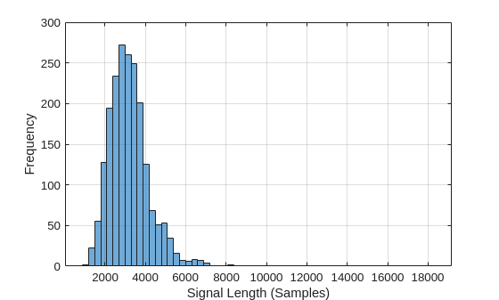
The histogram shows that the distribution of recording lengths is positively skewed. For classification, this example uses a common signal length of 8192 samples, a conservative value that ensures that truncating longer recordings does not cut off speech content. If the signal is greater than 8192 samples (1.024 seconds) in length, the recording is truncated to 8192 samples. If the signal is less than 8192 samples in length, the signal is prepadded and postpadded symmetrically with zeros out to a length of 8192 samples.
Wavelet Time Scattering
Use waveletScattering to create a wavelet time scattering framework using an invariant scale of 0.22 seconds. In this example, you create feature vectors by averaging the scattering transform over all time samples. To have a sufficient number of scattering coefficients per time window to average, set OversamplingFactor to 2 to produce a four-fold increase in the number of scattering coefficients for each path with respect to the critically downsampled value.
sf = waveletScattering(SignalLength=8192,InvarianceScale=0.22, ...
    SamplingFrequency=8000,OversamplingFactor=2);
Split the FSDD into training and test sets. Allocate 80% of the data to the training set and retain 20% for the test set. The training data is for training the classifier based on the scattering transform. The test data is for validating the model.
rng("default")
ads = shuffle(ads);
[adsTrain,adsTest] = splitEachLabel(ads,0.8);
countEachLabel(adsTrain)ans=10×2 table
0 160
1 160
2 160
3 160
4 160
5 160
6 160
7 160
8 160
9 160
countEachLabel(adsTest)
ans=10×2 table
    0    40
    1    40
    2    40
    3    40
    4    40
    5    40
    6    40
    7    40
    8    40
    9    40
The helper function helperReadSPData truncates or pads the data to a length of 8192 and normalizes each recording by its maximum value. The source code for helperReadSPData is listed in the appendix. Create an 8192-by-1600 matrix where each column is a spoken-digit recording.
Xtrain = [];
scatds_Train = transform(adsTrain,@(x)helperReadSPData(x));
while hasdata(scatds_Train)
    smat = read(scatds_Train);
    Xtrain = cat(2,Xtrain,smat);
end
Repeat the process for the test set. The resulting matrix is 8192-by-400.
Xtest = [];
scatds_Test = transform(adsTest,@(x)helperReadSPData(x));
while hasdata(scatds_Test)
    smat = read(scatds_Test);
    Xtest = cat(2,Xtest,smat);
end
Apply the wavelet scattering transform to the training and test sets.
Strain = sf.featureMatrix(Xtrain);
Stest = sf.featureMatrix(Xtest);
Obtain the mean scattering features for the training and test sets. Exclude the zeroth-order scattering coefficients.
TrainFeatures = Strain(2:end,:,:);
TrainFeatures = squeeze(mean(TrainFeatures,2))';
TestFeatures = Stest(2:end,:,:);
TestFeatures = squeeze(mean(TestFeatures,2))';
SVM Classifier
Now that the data has been reduced to a feature vector for each recording, the next step is to use these features for classifying the recordings. Create an SVM learner template with a quadratic polynomial kernel. Fit the SVM to the training data.
template = templateSVM(...
    KernelFunction="polynomial", ...
    PolynomialOrder=2, ...
    KernelScale="auto", ...
    BoxConstraint=1, ...
    Standardize=true);
classificationSVM = fitcecoc( ...
    TrainFeatures, ...
    adsTrain.Labels, ...
    Learners=template, ...
    Coding="onevsone", ...
    ClassNames=categorical({'0'; '1'; '2'; '3'; '4'; '5'; '6'; '7'; '8'; '9'}));
Use k-fold cross-validation to predict the generalization accuracy of the model based on the training data. Split the training set into five groups.
partitionedModel = crossval(classificationSVM,KFold=5);
[validationPredictions, validationScores] = kfoldPredict(partitionedModel);
validationAccuracy = (1 - kfoldLoss(partitionedModel,LossFun="ClassifError"))*100
validationAccuracy = 96.9375
The estimated generalization accuracy is approximately 97%. Use the trained SVM to predict the spoken-digit classes in the test set.
predLabels = predict(classificationSVM,TestFeatures);
testAccuracy = sum(predLabels==adsTest.Labels)/numel(predLabels)*100 %#ok<NASGU>
testAccuracy = 98
Summarize the performance of the model on the test set with a confusion chart. Display the precision and recall for each class by using column and row summaries. The table at the bottom of the confusion chart shows the precision values for each class. The table to the right of the confusion chart shows the recall values.
figure(Units="normalized",Position=[0.2 0.2 0.5 0.5])
ccscat = confusionchart(adsTest.Labels,predLabels);
ccscat.Title = "Wavelet Scattering Classification";
ccscat.ColumnSummary = "column-normalized";
ccscat.RowSummary = "row-normalized";

The scattering transform coupled with a SVM classifier classifies the spoken digits in the test set with an accuracy of 98% (or an error rate of 2%).
Long Short-Term Memory (LSTM) Networks
An LSTM network is a type of recurrent neural network (RNN). RNNs are neural networks that are specialized for working with sequential or temporal data such as speech data. Because the wavelet scattering coefficients are sequences, they can be used as inputs to an LSTM. By using scattering features as opposed to the raw data, you can reduce the variability that your network needs to learn.
Modify the training and testing scattering features to be used with the LSTM network. Exclude the zeroth-order scattering coefficients and convert the features to cell arrays.
TrainFeatures = Strain(2:end,:,:);
TrainFeatures = squeeze(num2cell(TrainFeatures,[1 2]));
TestFeatures = Stest(2:end,:,:);
TestFeatures = squeeze(num2cell(TestFeatures, [1 2]));
Construct a simple LSTM network with 256 hidden layers.
[inputSize, ~] = size(TrainFeatures{1});
YTrain = adsTrain.Labels;

numHiddenUnits = 256;
numClasses = numel(unique(YTrain));

layers = [ ...
    sequenceInputLayer(inputSize)
    lstmLayer(numHiddenUnits,OutputMode="last")
    fullyConnectedLayer(numClasses)
    softmaxLayer];
Set the hyperparameters. Use Adam optimization and a mini-batch size of 50. Set the maximum number of epochs to 300. Use a learning rate of 1e-4. You can turn off the training progress plot if you do not want to track the progress using plots. The training uses a GPU by default if one is available. Otherwise, it uses a CPU. For more information, see trainingOptions (Deep Learning Toolbox).
maxEpochs = 300;
miniBatchSize = 50;

options = trainingOptions("adam", ...
    InitialLearnRate=1e-4,...
    MaxEpochs=maxEpochs, ...
    MiniBatchSize=miniBatchSize, ...
    SequenceLength="shortest", ...
    Shuffle="every-epoch",...
    Verbose=false, ...
    Plots="training-progress", ...
    Metrics="accuracy", ...
    InputDataFormats="CTB");
Train the network.
net = trainnet(TrainFeatures,YTrain,layers,"crossentropy",options);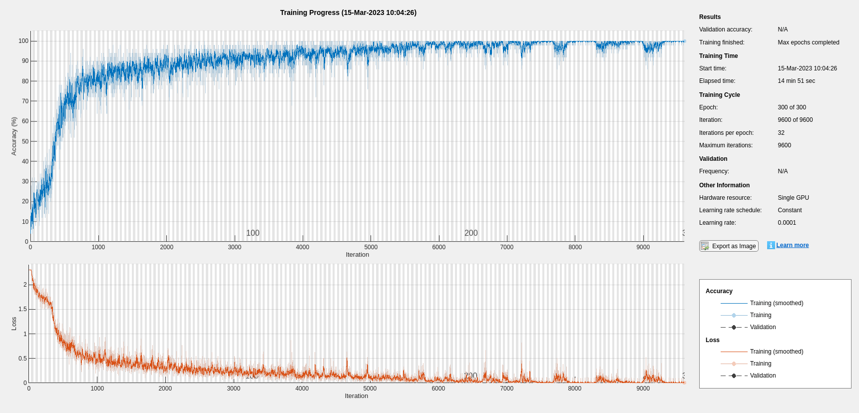
scores = minibatchpredict(net,TestFeatures,InputDataFormats="CTB");
classNames = categories(ads.Labels);
predLabels = scores2label(scores,classNames);
testAccuracy = sum(predLabels==adsTest.Labels)/numel(predLabels)*100 %#ok<NASGU>
testAccuracy =
93.7500
Bayesian Optimization
Determining suitable hyperparameter settings is often one of the most difficult parts of training a deep network. To mitigate this, you can use Bayesian optimization. In this example, you optimize the number of hidden layers and the initial learning rate by using Bayesian techniques. Create a new directory to store the MAT-files containing information about hyperparameter settings and the network along with the corresponding error rates.
YTrain = adsTrain.Labels;
YTest = adsTest.Labels;

if ~exist("results/",'dir')
    mkdir results
end
Initialize the variables to be optimized and their value ranges. Because the number of hidden layers must be an integer, set 'type' to 'integer'.
optVars = [
optimizableVariable(InitialLearnRate=[1e-5, 1e-2],Transform="log")
optimizableVariable(NumHiddenUnits=[100, 1000],Type="integer")
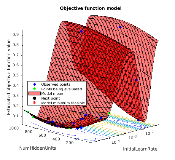
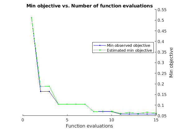
];Bayesian optimization is computationally intensive and can take several hours to finish. For the purposes of this example, set optimizeCondition to false to download and use predetermined optimized hyperparameter settings. If you set optimizeCondition to true, the objective function helperBayesOptLSTM is minimized using Bayesian optimization. The objective function, listed in the appendix, is the error rate of the network given specific hyperparameter settings. The loaded settings are for the objective function minimum of 0.02 (2% error rate).
ObjFcn = helperBayesOptLSTM(TrainFeatures,YTrain,TestFeatures,YTest);

optimizeCondition = false;
if optimizeCondition
    BayesObject = bayesopt(ObjFcn,optVars, ...
            MaxObjectiveEvaluations=15, ...
            IsObjectiveDeterministic=false, ...
            UseParallel=false); %#ok<UNRCH>
else
    url = "http://ssd.mathworks.com/supportfiles/audio/SpokenDigitRecognition.zip";
    downloadNetFolder = tempdir;
    netFolder = fullfile(downloadNetFolder,"SpokenDigitRecognition");
    if ~exist(netFolder,"dir")
        disp("Downloading pretrained network (1 file - 12 MB) ...")
        unzip(url,downloadNetFolder)
    end
    file = load(fullfile(netFolder,"0.02.mat"));
end
If you perform Bayesian optimization, figures similar to the following are generated to track the objective function values with the corresponding hyperparameter values and the number of iterations. You can increase the number of Bayesian optimization iterations to ensure that the global minimum of the objective function is reached.
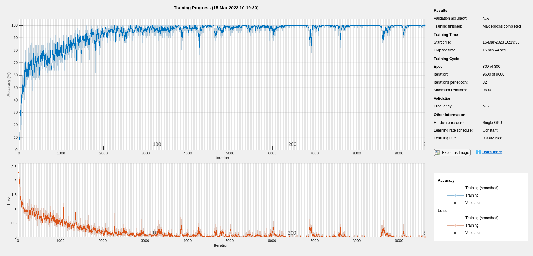
Use the optimized values for the number of hidden units and initial learning rate and retrain the network.
bestNumHiddenUnits = 768;
bestInitialLearnRate = 2.198827960269379e-04;


numClasses = numel(unique(YTrain));

layers = [ ...
    sequenceInputLayer(inputSize)
    lstmLayer(bestNumHiddenUnits,OutputMode="last")
    fullyConnectedLayer(numClasses)
    softmaxLayer];

maxEpochs = 300;
miniBatchSize = 50;

options = trainingOptions("adam", ...
    InitialLearnRate=bestInitialLearnRate, ...
    MaxEpochs=maxEpochs, ...
    MiniBatchSize=miniBatchSize, ...
    SequenceLength="shortest", ...
    Shuffle="every-epoch", ...
    Verbose=false, ...
    Plots="training-progress", ...
    Metrics="accuracy", ...
    InputDataFormats="CTB");

net = trainnet(TrainFeatures,YTrain,layers,"crossentropy",options);
scores = minibatchpredict(net,TestFeatures,InputDataFormats="CTB");
classNames = categories(ads.Labels);
predLabels = scores2label(scores,classNames);
testAccuracy = sum(predLabels==adsTest.Labels)/numel(predLabels)*100
testAccuracy = 97.5000
As the plot shows, using Bayesian optimization yields an LSTM with a higher accuracy.
Deep Convolutional Network Using Mel-Frequency Spectrograms
As another approach to the task of spoken digit recognition, use a deep convolutional neural network (DCNN) based on mel-frequency spectrograms to classify the FSDD data set. Use the same signal truncation/padding procedure as in the scattering transform. Similarly, normalize each recording by dividing each signal sample by the maximum absolute value. For consistency, use the same training and test sets as for the scattering transform.
Set the parameters for the mel-frequency spectrograms. Use the same window, or frame, duration as in the scattering transform, 0.22 seconds. Set the hop between windows to 10 ms. Use 40 frequency bands.
segmentDuration = 8192*(1/8000);
frameDuration = 0.22;
hopDuration = 0.01;
numBands = 40;
Reset the training and test datastores.
reset(adsTrain)
reset(adsTest)
The helper function helperspeechSpectrograms, defined at the end of this example, uses melSpectrogram (Audio Toolbox) to obtain the mel-frequency spectrogram after standardizing the recording length and normalizing the amplitude. Use the logarithm of the mel-frequency spectrograms as the inputs to the DCNN. To avoid taking the logarithm of zero, add a small epsilon to each element.
epsil = 1e-6;
XTrain = helperspeechSpectrograms(adsTrain,segmentDuration,frameDuration,hopDuration,numBands);
Computing speech spectrograms...
Processed 500 files out of 1600
Processed 1000 files out of 1600
Processed 1500 files out of 1600
...done
XTrain = log10(XTrain + epsil);

XTest = helperspeechSpectrograms(adsTest,segmentDuration,frameDuration,hopDuration,numBands);
Computing speech spectrograms...
...done
XTest = log10(XTest + epsil);

YTrain = adsTrain.Labels;
YTest = adsTest.Labels;
Define DCNN Architecture
Construct a small DCNN as an array of layers. Use convolutional and batch normalization layers, and downsample the feature maps using max pooling layers. To reduce the possibility of the network memorizing specific features of the training data, add a small amount of dropout to the input to the last fully connected layer.
sz = size(XTrain);
specSize = sz(1:2);
imageSize = [specSize 1];

numClasses = numel(categories(YTrain));

dropoutProb = 0.2;
numF = 12;
layers = [
    imageInputLayer(imageSize)

    convolution2dLayer(5,numF,Padding="same")
    batchNormalizationLayer
    reluLayer

    maxPooling2dLayer(3,Stride=2,Padding="same")

    convolution2dLayer(3,2*numF,Padding="same")
    batchNormalizationLayer
    reluLayer

    maxPooling2dLayer(3,Stride=2,Padding="same")

    convolution2dLayer(3,4*numF,Padding="same")
    batchNormalizationLayer
    reluLayer

    maxPooling2dLayer(3,Stride=2,Padding="same")

    convolution2dLayer(3,4*numF,Padding="same")
    batchNormalizationLayer
    reluLayer
    convolution2dLayer(3,4*numF,Padding="same")
    batchNormalizationLayer
    reluLayer

    maxPooling2dLayer(2)

    dropoutLayer(dropoutProb)
    fullyConnectedLayer(numClasses)
    softmaxLayer
    ];
Set the hyperparameters to use in training the network. Use a mini-batch size of 50 and a learning rate of 1e-4. Specify Adam optimization. You can train the network on an available GPU by setting the execution environment to either "gpu" or "auto". For more information, see trainingOptions (Deep Learning Toolbox).
miniBatchSize = 50;
options = trainingOptions("adam", ...
    InitialLearnRate=1e-4, ...
    MaxEpochs=30, ...
    MiniBatchSize=miniBatchSize, ...
    Shuffle="every-epoch", ...
    Plots="training-progress", ...
    Verbose=false, ...
    Metrics="accuracy", ...
    ExecutionEnvironment="auto");
Train the network.
trainedNet = trainnet(XTrain,YTrain,layers,"crossentropy",options);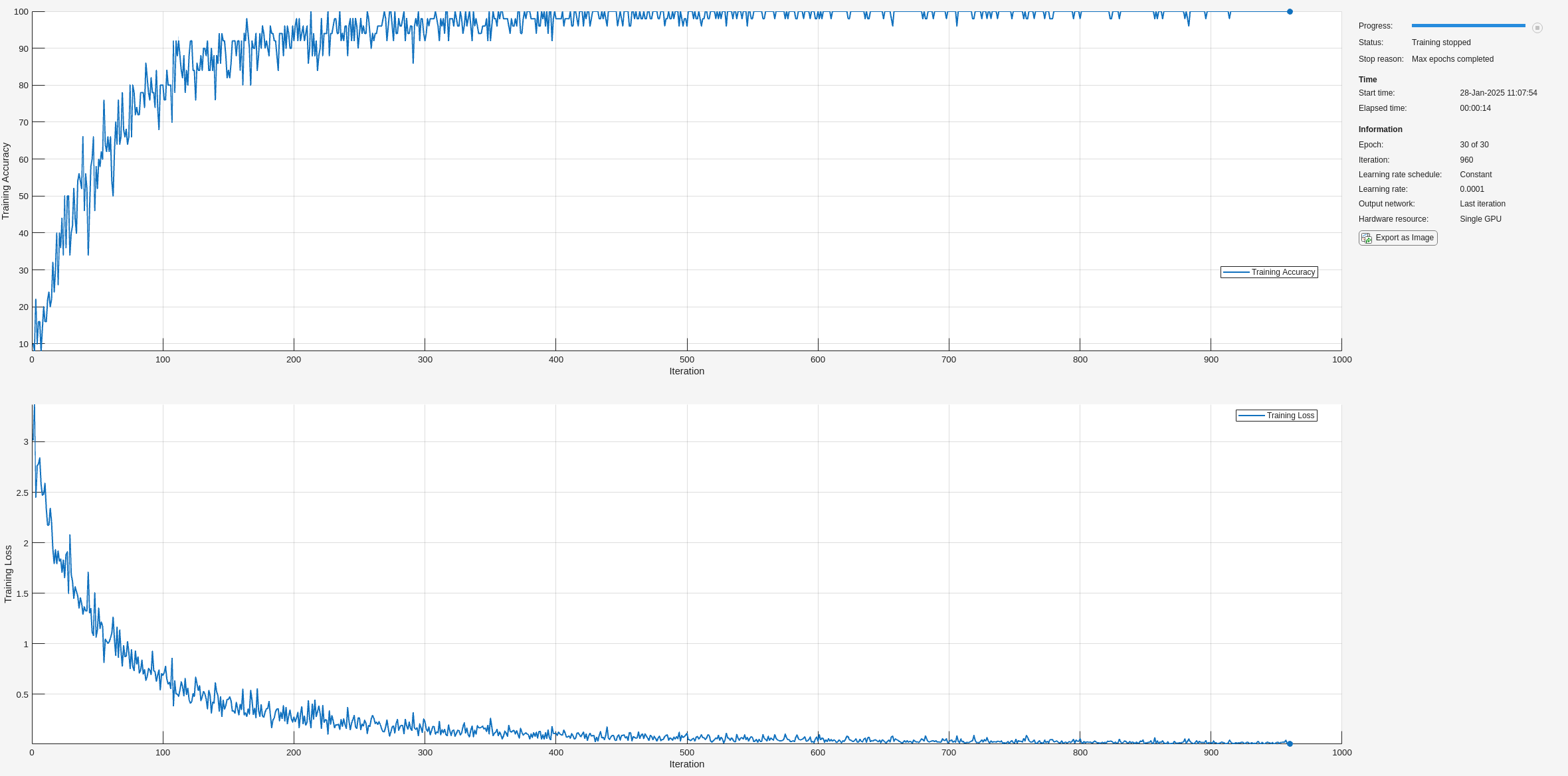
Use the trained network to predict the digit labels for the test set.
scores = minibatchpredict(trainedNet,XTest);
classNames = categories(YTrain);
Ypredicted = scores2label(scores,classNames);
cnnAccuracy = sum(Ypredicted==YTest)/numel(YTest)*100
cnnAccuracy =
98.7500
Summarize the performance of the trained network on the test set with a confusion chart. Display the precision and recall for each class by using column and row summaries. The table at the bottom of the confusion chart shows the precision values. The table to the right of the confusion chart shows the recall values.
figure(Units="normalized",Position=[0.2 0.2 0.5 0.5]);
ccDCNN = confusionchart(YTest,Ypredicted);
ccDCNN.Title = "Confusion Chart for DCNN";
ccDCNN.ColumnSummary = "column-normalized";
ccDCNN.RowSummary = "row-normalized";
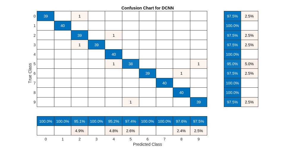
The DCNN using mel-frequency spectrograms as inputs classifies the spoken digits in the test set with an accuracy rate of approximately 98% as well.
Summary
This example shows how to use different machine and deep learning approaches for classifying spoken digits in the FSDD. The example illustrated wavelet scattering paired with both an SVM and a LSTM. Bayesian techniques were used to optimize LSTM hyperparameters. Finally, the example shows how to use a CNN with mel-frequency spectrograms.
The goal of the example is to demonstrate how to use MathWorks® tools to approach the problem in fundamentally different but complementary ways. All workflows use audioDatastore to manage flow of data from disk and ensure proper randomization.
All approaches used in this example performed equally well on the test set. This example is not intended as a direct comparison between the various approaches. For example, you can also use Bayesian optimization for hyperparameter selection in the CNN. An additional strategy that is useful in deep learning with small training sets like this version of the FSDD is to use data augmentation. How manipulations affect class is not always known, so data augmentation is not always feasible. However, for speech, established data augmentation strategies are available through audioDataAugmenter (Audio Toolbox).
In the case of wavelet time scattering, there are also a number of modifications you can try. For example, you can change the invariant scale of the transform, vary the number of wavelet filters per filter bank, and try different classifiers.
Appendix: Helper Functions
function Labels = helpergenLabels(ads)
% This function is only for use in Wavelet Toolbox examples. It may be
% changed or removed in a future release.
tmp = cell(numel(ads.Files),1);
expression = "[0-9]+_";
for nf = 1:numel(ads.Files)
    idx = regexp(ads.Files{nf},expression);
    tmp{nf} = ads.Files{nf}(idx);
end
Labels = categorical(tmp);
end
function x = helperReadSPData(x)
% This function is only for use Wavelet Toolbox examples. It may change or
% be removed in a future release.

N = numel(x);
if N > 8192
    x = x(1:8192);
elseif N < 8192
    pad = 8192-N;
    prepad = floor(pad/2);
    postpad = ceil(pad/2);
    x = [zeros(prepad,1) ; x ; zeros(postpad,1)];
end
x = x./max(abs(x));

end
function x = helperBayesOptLSTM(X_train, Y_train, X_val, Y_val)
% This function is only for use in the
% "Spoken Digit Recognition with Wavelet Scattering and Deep Learning"
% example. It may change or be removed in a future release.
x = @valErrorFun;

    function [valError,cons, fileName] = valErrorFun(optVars)
        %% LSTM Architecture
        [inputSize,~] = size(X_train{1});
        numClasses = numel(unique(Y_train));

        layers = [ ...
            sequenceInputLayer(inputSize)
            bilstmLayer(optVars.NumHiddenUnits,OutputMode="last") % Using number of hidden layers value from optimizing variable
            fullyConnectedLayer(numClasses)
            softmaxLayer];

        % Plots not displayed during training
        options = trainingOptions("adam", ...
            InitialLearnRate=optVars.InitialLearnRate, ... % Using initial learning rate value from optimizing variable
            MaxEpochs=300, ...
            MiniBatchSize=30, ...
            SequenceLength="shortest", ...
            Shuffle="every-epoch", ...
            Verbose=false, ...
            Metrics="accuracy", ...
            InputDataFormats="CTB");

        %% Train the network
        net = trainnet(X_train, Y_train, layers, "crossentropy", options);
        %% Training accuracy
        scores = minibatchpredict(net,X_val,InputDataFormats="CTB");
        classNames = categories(Y_train);
        X_val_P = scores2label(scores,classNames);
        accuracy_training  = sum(X_val_P == Y_val)./numel(Y_val);
        valError = 1 - accuracy_training;
        %% save results of network and options in a MAT file in the results folder along with the error value
        fileName = fullfile("results", num2str(valError) + ".mat");
        save(fileName,"net","valError","options")
        cons = [];
    end % end for inner function
end % end for outer function
function X = helperspeechSpectrograms(ads,segmentDuration,frameDuration,hopDuration,numBands)
% This function is only for use in the
% "Spoken Digit Recognition with Wavelet Scattering and Deep Learning"
% example. It may change or be removed in a future release.
%
% helperspeechSpectrograms(ads,segmentDuration,frameDuration,hopDuration,numBands)
% computes speech spectrograms for the files in the datastore ads.
% segmentDuration is the total duration of the speech clips (in seconds),
% frameDuration the duration of each spectrogram frame, hopDuration the
% time shift between each spectrogram frame, and numBands the number of
% frequency bands.
disp("Computing speech spectrograms...");

numHops = ceil((segmentDuration - frameDuration)/hopDuration);
numFiles = length(ads.Files);
X = zeros([numBands,numHops,1,numFiles],"single");

for i = 1:numFiles

    [x,info] = read(ads);
    x = normalizeAndResize(x);
    fs = info.SampleRate;
    frameLength = round(frameDuration*fs);
    hopLength = round(hopDuration*fs);

    spec = melSpectrogram(x,fs, ...
        Window=hamming(frameLength,"periodic"), ...
        OverlapLength=frameLength-hopLength, ...
        FFTLength=2048, ...
        NumBands=numBands, ...
        FrequencyRange=[50,4000]);

    % If the spectrogram is less wide than numHops, then put spectrogram in
    % the middle of X.
    w = size(spec,2);
    left = floor((numHops-w)/2)+1;
    ind = left:left+w-1;
    X(:,ind,1,i) = spec;

    if mod(i,500) == 0
        disp("Processed " + i + " files out of " + numFiles)
    end

end

disp("...done");

end

%--------------------------------------------------------------------------
function x = normalizeAndResize(x)
% This function is only for use in the
% "Spoken Digit Recognition with Wavelet Scattering and Deep Learning"
% example. It may change or be removed in a future release.

N = numel(x);
if N > 8192
    x = x(1:8192);
elseif N < 8192
    pad = 8192-N;
    prepad = floor(pad/2);
    postpad = ceil(pad/2);
    x = [zeros(prepad,1) ; x ; zeros(postpad,1)];
end
x = x./max(abs(x));
end
References
[1] Jakobovski. “Jakobovski/Free-Spoken-Digit-Dataset.” GitHub, May 30, 2019. https://github.com/Jakobovski/free-spoken-digit-dataset.
Copyright 2018-2025, The MathWorks, Inc.
See Also
Objects
waveletScattering|audioDatastore(Audio Toolbox) |audioDataAugmenter(Audio Toolbox)
Functions
featureMatrix|melSpectrogram(Audio Toolbox)