Visualize and Recreate VMD Decomposition

This example shows how to visualize the intrinsic mode functions and residual of a variational mode decomposition (VMD) using Signal Multiresolution Analyzer. You learn how to compare two different decompositions in the app, and how to recreate a decomposition in your workspace.

Generate a piecewise composite signal consisting of a quadratic trend, a chirp, and a cosine with a sharp transition between two constant frequencies at t = 0.5. Sample the signal for 1 second at 1000 Hz. Plot the signal.

$$x(t)=6t^2+\cos (4\pi t+10\pi t^2)+\{\begin{array}{ll}\cos (60\pi t),& t\le 0.5,\\ \cos (100\pi t-10\pi ),& t>0.5.\end{array}$$

fs = 1e3;
t = 0:1/fs:1-1/fs;

sig = 6*t.^2 + cos(4*pi*t+10*pi*t.^2) + ...
    [cos(60*pi*(t(t<=0.5))) cos(100*pi*(t(t>0.5)-10*pi))];

plot(t,sig)
title("Signal")
xlabel("Time (s)")
ylabel("Amplitude")

Visualize VMD

Open Signal Multiresolution Analyzer and click Import. Select sig and click Import. By default, a four-level MODWTMRA decomposition appears in the MODWT tab. In the Signal Multiresolution Analyzer tab, set the sample rate to 1000 Hz.

To generate a variational mode decomposition of the signal, go to the Signal Multiresolution Analyzer tab. Click Add ▼ and select VMD.

After a few moments, the VMD decomposition sig2 appears in the VMD tab. The app obtains the decomposition using the vmd function with default settings. The Level Selection pane shows the relative energies of the signal across the intrinsic mode functions (IMF), as well as the measured frequency ranges. With the toolstrip, you can change the VMD parameters to generate a different decomposition. You can specify:

• Number of IMFs extracted

• Mode convergence relative and absolute tolerances

• Maximum number of optimization iterations

• Initial IMFs

• Initial Lagrange multiplier and update rate for the Lagrange multiplier in each iteration

• Method to initialize the central frequencies

• Penalty factor that determines the reconstruction fidelity

Changing a value enables the Decompose button. To learn more about the parameters, see vmd.

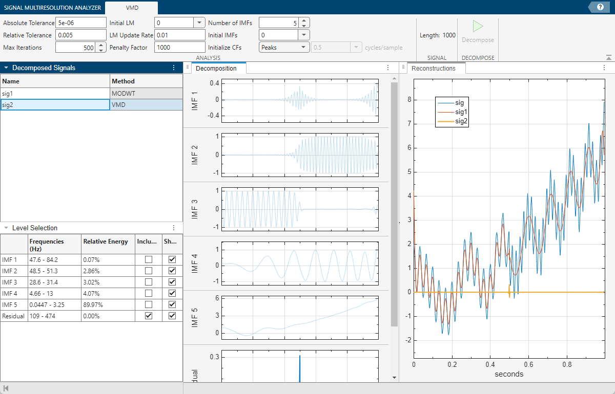
Set the number of extracted IMFs to 4 and click Decompose to visualize the decomposition. The app recovers four distinct components of the signal. Include the first and fourth IMFs in the reconstruction.

Export Script

To recreate the decomposition in your workspace, in the Signal Multiresolution Analyzer tab click Export > Generate MATLAB Script. An untitled script opens in your editor with the following executable code. The true-false values in levelForReconstruction correspond to the Include boxes you selected in the Level Selection pane. You can save the script as is or modify it to apply the same decomposition settings to other signals. Run the code.

% Logical array for selecting reconstruction elements
levelForReconstruction = [true,false,false,true,true];

% Perform the decomposition using VMD
[imf,residual,info] = vmd(sig, ...
    AbsoluteTolerance=5e-06, ...
    RelativeTolerance=0.005, ...
    MaxIterations=500, ...
    NumIMF=4, ...
    InitialIMFs=zeros(1000,4), ...
    PenaltyFactor=1000, ...
    InitialLM=complex(zeros(1001,1)), ...
    LMUpdateRate=0.01, ...
    InitializeMethod='peaks');

% Construct MRA matrix by appending IMFs and residual
mra = [imf residual].';

% Sum down the rows of the selected multiresolution signals
sig2 = sum(mra(levelForReconstruction,:),1);

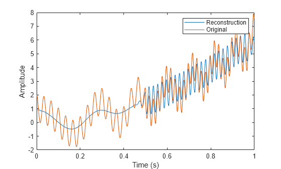
The rows in the MRA matrix mra correspond to the IMFs and residual in the Level Selection pane. Plot the reconstruction, which consists of the residual and two IMFs, and compare with the original signal.

plot(t,sig2)
hold on
plot(t,sig)
hold off
legend("Reconstruction","Original")
xlabel("Time (s)")
ylabel("Amplitude")

References

[1] Dragomiretskiy, Konstantin, and Dominique Zosso. “Variational Mode Decomposition.” IEEE Transactions on Signal Processing 62, no. 3 (February 2014): 531–44. https://doi.org/10.1109/TSP.2013.2288675.