Results for
Giving All Your Claudes the Keys to Everything
Introduction
This started as a plumbing problem. I wanted to move files between Claude’s cloud container and my Mac faster than base64 encoding allows. What I ended up building was something more interesting: a way for every Claude – Desktop, web browser, iPhone – to control my entire computing environment with natural language. MATLAB, Keynote, LaTeX, Chrome, Safari, my file system, text-to-speech. All of it, from any device, through a 200-line Python server and a free tunnel.
It isn’t quite the ideal universal remote. Web and iPhone Claude do not yet have the agentic Playwright-based web automation capabilities available to Claude desktop via MCP. A possible solution may be explored in a later post.
Background information
The background here is a series of experiments I’ve been running on giving AI desktop apps direct access to local tools. See How to set up and use AI Desktop Apps with MATLAB and MCP servers which covers the initial MCP setup, A universal agentic AI for your laptop and beyond which describes what Desktop Claude can do once you give it the keys, and Web automation with Claude, MATLAB, Chromium, and Playwright which describes a supercharged browser assistant. This post is about giving such keys to remote Claude interfaces.
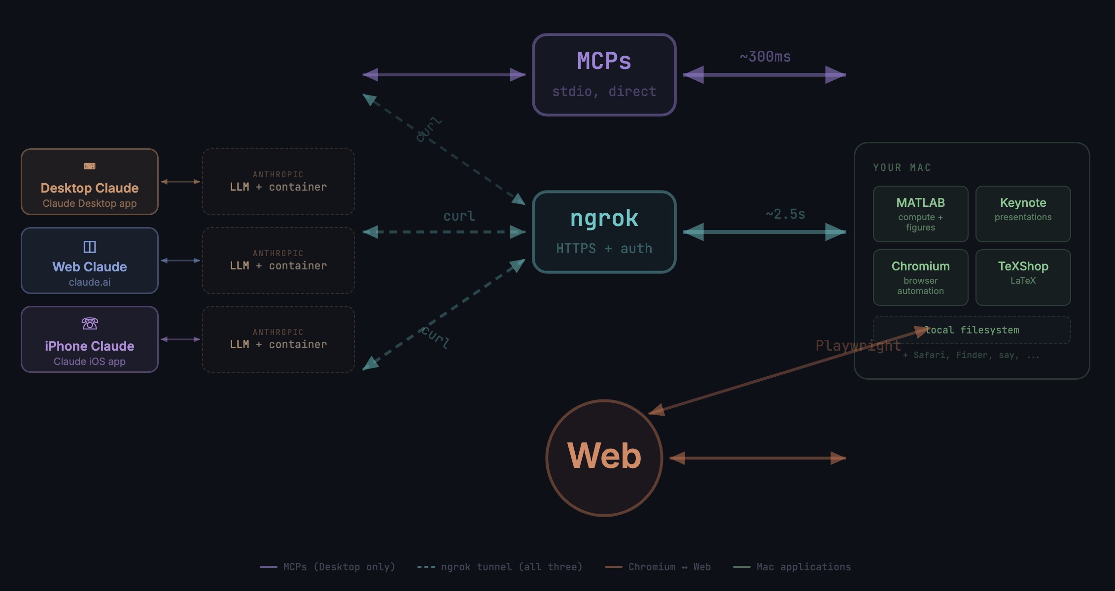
Through the Model Context Protocol (MCP), Claude Desktop on my Mac can run MATLAB code, read and write files, execute shell commands, control applications via AppleScript, automate browsers with Playwright, control iPhone apps, and take screenshots. These powers have been limited to the desktop Claude app – the one running on the machine with the MCP servers. My iPhone Claude app and a Claude chat launched in a browser interface each have a Linux container somewhere in Anthropic’s cloud. The container can reach the public internet. Until now, my Mac sat behind a home router with no public IP.
An HTTP server MCP replacement
A solution is a small HTTP server on the Mac. Use ngrok (free tier) to give the Mac a public URL. Then anything with internet access – including any Claude’s cloud container – can reach the Mac via curl.
iPhone/Web Claude -> bash_tool: curl https://public-url/endpoint
-> Internet -> ngrok tunnel -> Mac localhost:8765
-> Python command server -> MATLAB / AppleScript / filesystem
The server is about 200 lines of Python using only the standard library. Two files, one terminal command to start. ngrok provides HTTPS and HTTP Basic Auth with a single command-line flag.
The complete implementation consists of three files:
claude_command_server.py (~200 lines): A Python HTTP server using http.server from the standard library. It implements BaseHTTPRequestHandler with do_GET and do_POST methods dispatching to endpoint handlers. Shell commands are executed via subprocess.run with timeout protection. File paths are validated against allowed roots using os.path.realpath to prevent directory traversal attacks.
start_claude_server.sh (~20 lines): A Bash script that starts the Python server as a background process, then starts ngrok in the foreground. A trap handler ensures both processes are killed on Ctrl+C.
iphone_matlab_watcher.m (~60 lines): MATLAB timer function that polls for command files every second.
The server exposes six GET and six POST endpoints. The GET endpoints thus far handle retrieval: /ping for health checks, /list to enumerate files in a transfer directory, /files/<n> to download a file from that directory, /read/<path> to read any file under allowed directories, and / which returns the endpoint listing itself. The POST endpoints handle execution and writing: /shell runs an allowlisted shell command, /osascript runs AppleScript, /matlab evaluates MATLAB code through a file-watcher mechanism, /screenshot captures the screen and returns a compressed JPEG, /write writes content to a file, and /upload/<n> accepts binary uploads.
File access is sandboxed by endpoint. The /read/ endpoint restricts reads to ~/Documents, ~/Downloads, and ~/Desktop and their subfolders. The /write and /upload endpoints restrict writes to ~/Documents/MATLAB and ~/Downloads. Path traversal is validated – .. sequences are rejected.
The /shell endpoint restricts commands to an explicit allowlist: open, ls, cat, head, tail, cp, mv, mkdir, touch, find, grep, wc, file, date, which, ps, screencapture, sips, convert, zip, unzip, pbcopy, pbpaste, say, mdfind, and curl. No rm, no sudo, no arbitrary execution. Content creation goes through /write.
Two endpoints have no path restrictions: /osascript and /matlab. The /osascript endpoint passes its payload to macOS’s osascript command, which executes AppleScript – Apple’s scripting language for controlling applications via inter-process Apple Events. An AppleScript can open, close, or manipulate any application, read or write any file the user account can access, and execute arbitrary shell commands via “do shell script”. The /matlab endpoint evaluates arbitrary MATLAB code in a persistent session. Both are as powerful as the user account itself. This is deliberate – these are the endpoints that make the server useful for controlling applications. The security boundary is authentication at the tunnel, not restriction at the endpoint.
The MATLAB Workaround
MATLAB on macOS doesn’t expose an AppleScript interface, and the MCP MATLAB tool uses a stdio connection available only from Desktop. So how does iPhone Claude run MATLAB?
An answer is a file-based polling mechanism. A MATLAB timer function checks a designated folder every second for new command files. The remote Claude writes a .m file via the server, MATLAB executes it, writes output to a text file, and sets a completion flag. The round trip is about 2.5 seconds including up to 1 second of polling latency. (This could be reduced by shortening the polling interval or replacing it with Java’s WatchService for near-instant file detection.)
This method provides full MATLAB access from a phone or web Claude, with your local file system available, under AI control. MATLAB Mobile and MATLAB Online do not offer agentic AI access.
Alternate approaches
I’ve used Tailscale Funnel as an alternative tunnel to manually control my MacBook from iPhone but you can’t install Tailscale inside Anthropic’s container. An alternative approach would replace both the local MCP servers and the command server with a single remote MCP server running on the Mac, exposed via ngrok and registered as a custom connector in claude.ai. This would give all three Claude interfaces native MCP tool access including Playwright or Puppeteer with comparable latency but I’ve not tried this.
Security
Exposing a command server to the internet raises questions. The security model has several layers. ngrok handles authentication – every request needs a valid password. Shell commands are restricted to an allowlist (ls, cat, cp, screencapture – no rm, no arbitrary execution). File operations are sandboxed to specific directory trees with path traversal validation. The server binds to localhost, unreachable without the tunnel. And you only run it when you need it.
The AppleScript and MATLAB endpoints are relatively unrestricted in my setup, giving Claude Desktop significant capabilities via MCP. Extending them through an authenticated tunnel is a trust decision.
Initial test results
I ran an identical three-step benchmark from each Claude interface: get a Mac timestamp via AppleScript, compute eigenvalues of a 10x10 magic square in MATLAB, and capture a screenshot. Same Mac, same server, same operations.
| Step | Desktop (MCP) | Web Claude | iPhone Claude |
|------|:------------:|:----------:|:-------------:|
| AppleScript timestamp | ~5ms | 626ms | 623ms |
| MATLAB eig(magic(10)) | 108ms | 833ms | 1,451ms |
| Screenshot capture | ~200ms | 1,172ms | 980ms |
| **Total** | **~313ms** | **2,663ms** | **3,078ms** |
The network overhead is consistent: web and iPhone both add about 620ms per call (the ngrok round trip through residential internet). Desktop MCP has no network overhead at all. The MATLAB variance between web (833ms) and iPhone (1,451ms) is mostly the file-watcher polling jitter – up to a second of random latency depending on where in the polling cycle the command arrives.
All three Claudes got the correct eigenvalues. All three controlled the Mac. The slowest total was 3 seconds for three separate operations from a phone. Desktop is 10x faster, but for “I’m on my phone and need to run something” – 3 seconds is fine.
Other tests
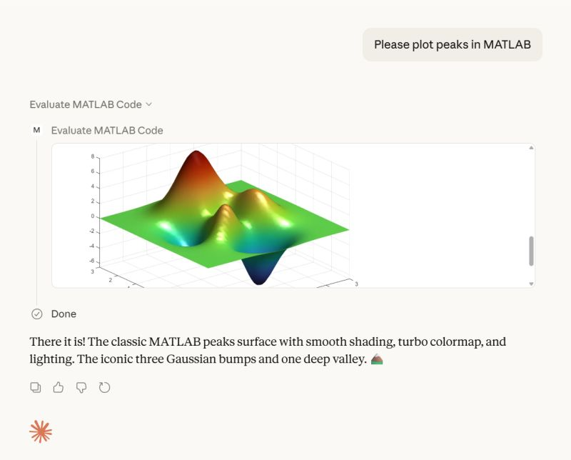
MATLAB: Computations (determinants, eigenvalues), 3D figure generation, image compression. The complete pipeline – compute on Mac, transfer figure to cloud, process with Python, send back – runs in under 5 seconds. This was previously impossible; there was no reasonable mechanism to move a binary file from the container to the Mac.
Keynote: Built multi-slide presentations via AppleScript, screenshotted the results.
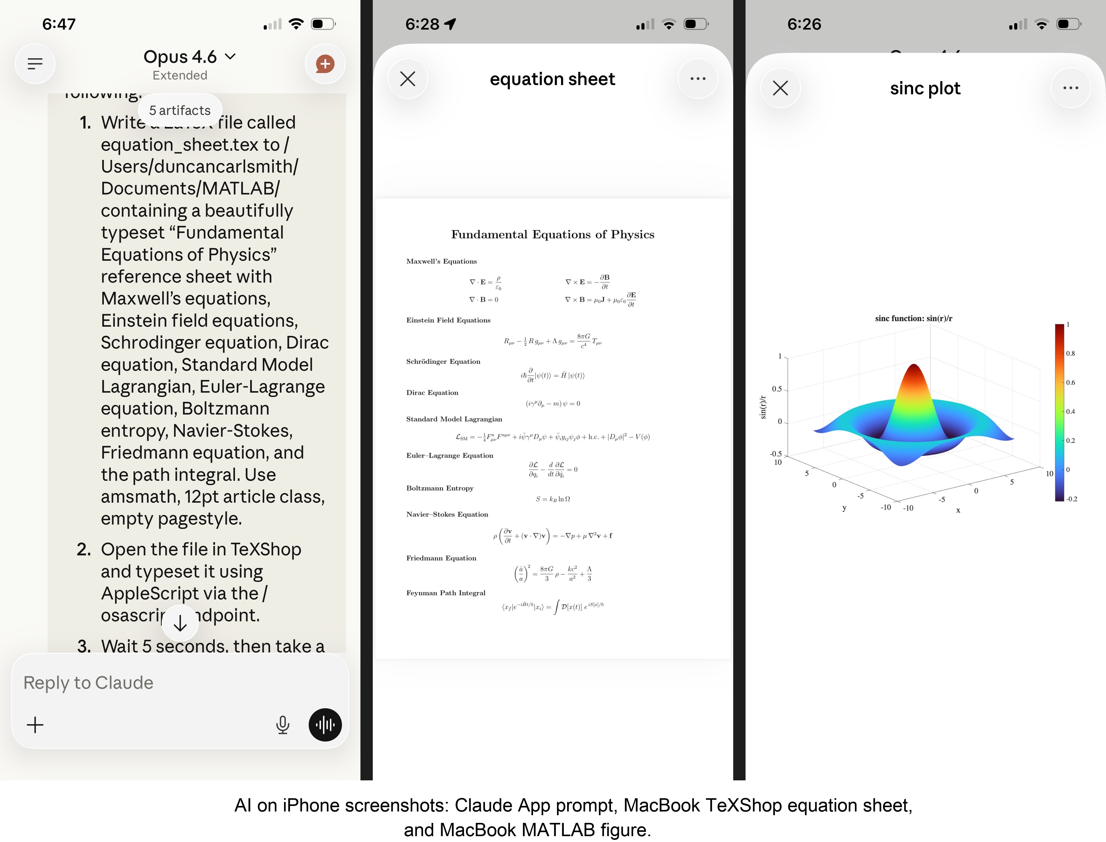
TeXShop: Wrote a .tex file containing ten fundamental physics equations (Maxwell through the path integral), opened it in TeXShop, typeset via AppleScript, captured the rendered PDF. Publication-quality typesetting from a phone. I don’t know who needs this at 11 PM on a Sunday, but apparently I do.
Safari: Launched URLs on the Mac from 2,000 miles away. Or 6 feet. The internet doesn’t care.
Finder: Directory listings, file operations, the usual filesystem work.
Text-to-speech: Mac spoke “Hello from iPhone” and “Web Claude is alive” on command. Silly but satisfying proof of concept.
File Transfer: The Original Problem, Solved
Remember, this started because I wanted faster file transfers for desktop Claude. Compare:
| Method | 1 MB file | 5 MB file | Limit |
|--------|-----------|-----------|-------|
| Old (base64 in context) | painful | impossible | ~5 KB |
| Command server upload | 455ms | ~3.6s | tested to 5 MB+ |
| Command server download | 1,404ms | ~7s | tested to 5 MB+ |
The improvement is the difference between “doesn’t work” and “works in seconds.”
Cross-Device Memory
A nice bonus: iPhone and web Claudes can search Desktop conversations using the same memory tools. Context established in a Desktop session – including the server password – can be retrieved from a phone conversation. You do have to ask explicitly (“search my past conversations for the command server”) or insert information into the persistent context using settings rather than assuming Claude will look on its own.
Web Claudes
The most surprising result was web Claude. I expected it to work – same container infrastructure, same bash_tool, same curl. But “expected to work” and “just worked, first try, no special setup” are different things. I opened claude.ai in a browser, gave it the server URL and password, and it immediately ran MATLAB, took screenshots, and made my Mac speak. No configuration, no troubleshooting, no “the endpoint format is wrong” iterations. If you’re logged into claude.ai and the server is running, you have full Mac access from any browser on any device.
What This Means
MCP gave Desktop Claude the keys to my Mac. A 200-line server and a free tunnel duplicated those keys for every other Claude I use. Three interfaces, one Mac, all the same applications, all controlled in natural language.
Additional information
An appendix gives Claude’s detailed description of communications. Codes and instructions are available at the MATLAB File Exchange: Giving All Your Claudes the Keys to Everything.
Acknowledgments and disclaimer
The problem of file transfer was identified by the author. Claude suggested and implemented the method, and the author suggested the generalization to accommodate remote Claudes. This submission was created with Claude assistance. The author has no financial interest in Anthropic or MathWorks.
—————
Appendix: Architecture Comparison
Path A: Desktop Claude with a Local MCP Server
When you type a message in the Desktop Claude app, the Electron app sends it to Anthropic’s API over HTTPS. The LLM processes the message and decides it needs a tool – say, browser_navigate from Playwright. It returns a tool_use block with the tool name and arguments. That block comes back to the Desktop app over the same HTTPS connection.
Here is where the local MCP path kicks in. At startup, the Desktop app read claude_desktop_config.json, found each MCP server entry, and spawned it as a child process on your Mac. It performed a JSON-RPC initialize handshake with each one, then called tools/list to get the tool catalog – names, descriptions, parameter schemas. All those tools were merged and sent to Anthropic with your message, so the LLM knows what’s available.
When the tool_use block arrives, the Desktop app looks up which child process owns that tool and writes a JSON-RPC message to that process’s stdin. The MCP server (Playwright, MATLAB, whatever) reads the request, does the work locally, and writes the result back to stdout as JSON-RPC. The Desktop app reads the result, sends it back to Anthropic’s API, the LLM generates the final text response, and you see it.
The Desktop app is really just a process manager and JSON-RPC router. The config file is a registry of servers to spawn. You can plug in as many as you want – each is an independent child process advertising its own tools. The Desktop app doesn’t care what they do internally. The MCP execution itself adds almost no latency because it’s entirely local, process-to-process on your Mac. The time you perceive is dominated by the two HTTPS round-trips to Anthropic, which all three Claude interfaces share equally.
Path B: iPhone Claude with the Command Server
When you type a message in the Claude iOS app, the app sends it to Anthropic’s API over HTTPS, same as Desktop. The LLM processes the message. It sees bash_tool in its available tools – provided by Anthropic’s container infrastructure, not by any MCP server. It decides it needs to run a curl command and returns a tool_use block for bash_tool.
Here, the path diverges completely from Desktop. There is no iPhone app involvement in tool execution. Anthropic routes the tool_use to a Linux container running in Anthropic’s cloud, assigned to your conversation. This container is the “computer” that iPhone Claude has access to. The container runs the curl command – a real Linux process in Anthropic’s data center.
The curl request goes out over the internet to ngrok’s servers. ngrok forwards it through its persistent tunnel to the claude_command_server.py process running on localhost on your Mac. The command server authenticates the request (basic auth), then executes the requested operation – in this case, running an AppleScript via subprocess.run(['osascript', ...]). macOS receives the Apple Events, launches the target application, and does the work.
The result flows back the same way: osascript returns output to the command server, which packages it as JSON and sends the HTTP response back through the ngrok tunnel, through ngrok’s servers, back to the container’s curl process. bash_tool captures the output. The container sends the tool result back to Anthropic’s API. The LLM generates the text response, and the iPhone app displays it.
The iPhone app is a thin chat client. It never touches tool execution – it only sends and receives chat messages. The container does the curl work, and the command server bridges from Anthropic’s cloud to your Mac. The LLM has to know to use curl with the right URL, credentials, and JSON format. There is no tool discovery, no protocol handshake, no automatic routing. The knowledge of how to reach your Mac is carried entirely in the LLM’s context.
—————
Duncan Carlsmith, Department of Physics, University of Wisconsin-Madison. duncan.carlsmith@wisc.edu
Web Automation with Claude, MATLAB, Chromium, and Playwright
Duncan Carlsmith, University of Wisconsin-Madison
Introduction
Recent agentic browsers (Chrome with Claude Chrome extension and Comet by Perplexity) are marvelous but limited. This post describes two things: first, a personal agentic browser system that outperforms commercial AI browsers for complex tasks; and second, how to turn AI-discovered web workflows into free, deterministic MATLAB scripts that run without AI.
My setup is a MacBook Pro with the Claude Desktop app, MATLAB 2025b, and Chromium open-source browser. Relevant MCP servers include fetch, filesystem, MATLAB, and Playwright, with shell access via MATLAB or shell MCP. Rather than use my Desktop Chrome application, which might expose personal information, I use an independent, dedicated Chromium with a persistent login and preauthentication for protected websites. Rather than screenshots, which quickly saturate a chat context and are expensive, I use the Playwright MCP server, which accesses the browser DOM and accessibility tree directly. DOM manipulation permits error-free operation of complex web page UIs.
The toolchain required is straightforward. You need Node.js , which is the JavaScript runtime that executes Playwright scripts outside a browser. Install it, then set up a working directory and install Playwright with its bundled Chromium:
# Install Node.js via Homebrew (macOS) or download from nodejs.org
brew install node
# Create a working directory and install Playwright
mkdir MATLABWithPlaywright && cd MATLABWithPlaywright
npm init -y
npm install playwright
# Download Playwright's bundled Chromium (required for Tier 1)
npx playwright install chromium
That is sufficient for the Tier 1 examples. For Tier 2 (authenticated automation), you also need Google Chrome or the open-source Chromium browser, launched with remote debugging enabled as described below. Playwright itself is an open-source browser automation library from Microsoft that can either launch its own bundled browser or connect to an existing one -- this dual capability is the foundation of the two-tier architecture. For the AI-agentic work described in the Canvas section, you need Claude Desktop with MCP servers configured for filesystem access, MATLAB, and Playwright. The INSTALL.md in the accompanying FEX submission covers all of this in detail.
AI Browser on Steroids: Building Canvas Quizzes
An agentic browser example just completed illustrates the power of this approach. I am adding a computational thread to a Canvas LMS course in modern physics based on relevant interactive Live Scripts I have posted to the MATLAB File Exchange. For each of about 40 such Live Scripts, I wanted to build a Canvas quiz containing an introduction followed by a few multiple-choice questions and a few file-upload questions based on the "Try this" interactive suggestions (typically slider parameter adjustments) and "Challenges" (typically to extend the code to achieve some goal). The Canvas interface for quiz building is quite complex, especially since I use a lot of LaTeX, which in the LMS is rendered using MathJax with accessibility features and only a certain flavor of encoding works such that the math is rendered both in the quiz editor and when the quiz is displayed to a student.
My first prompt was essentially "Find all of my FEX submissions and categorize those relevant to modern physics.” The categories emerged as Relativity, Quantum Mechanics, Atomic Physics, and Astronomy and Astrophysics. Having preauthenticated at MathWorks with a Shibboleth university license authentication system, the next prompt was "Download and unzip the first submission in the relativity category, read the PDF of the executed script or view it under examples at FEX, then create quiz questions and answers as described above." The final prompt was essentially "Create a new quiz in my Canvas course in the Computation category with a due date at the end of the semester. Include the image and introduction from the FEX splash page and a link to FEX in the quiz instructions. Add the MC quiz questions with 4 answers each to select from, and the file upload questions. Record what you learned in a SKILL file in my MATLAB/claude/SKILLS folder on my filesystem." Claude offered a few options, and we chose to write and upload the quiz HTML from scratch via the Canvas REST API. Done. Finally, "Repeat for the other FEX File submissions." Each took a couple of minutes. The hard part was figuring out what I wanted to do exactly.
Mind you, I had tried to build a Canvas quiz including LaTeX and failed miserably with both Chrome Extension and Comet. The UI manipulations, especially to handle the LaTeX, were too complex, and often these agentic browsers would click in the wrong place, wind up on a different page, even in another tab, and potentially become destructive.
A key gotcha with LaTeX in Canvas: the equation rendering system uses double URL encoding for LaTeX expressions embedded as image tags pointing to the Canvas equation server. The LaTeX strings must use single backslashes -- double backslashes produce broken output. And Canvas Classic Quizzes and New Quizzes handle MathJax differently, so you need to know which flavor your institution uses.
From AI-Assisted to Programmatic: The Two-Tier Architecture
An agentic-AI process, like the quiz creation, can become expensive. There is a lot of context, both physics content-related and process-related, and the token load mounts up in a chat. Wouldn't it be great if, after having used the AI for what it is best at -- summarizing material, designing student exercises, and discovering a web-automation process -- one could repeat the web-related steps programmatically for free with MATLAB? Indeed, it would, and is.
In my setup, usually an AI uses MATLAB MCP to operate MATLAB as a tool to assist with, say, launching an application like Chromium or to preprocess an image. But MATLAB can also launch any browser and operate it via Playwright. (To my knowledge, MATLAB can use its own browser to view a URL but not to manipulate it.) So the following workflow emerges:
1) Use an AI, perhaps by recording the DOM steps in a manual (human) manipulation, to discover a web-automation process.
2) Use the AI to write and debug MATLAB code to perform the process repeatedly, automatically, for free.
I call this "temperature zero" automation -- the AI contributes entropy during workflow discovery, then the deterministic script is the ground state.
The architecture has three layers:
MATLAB function (.m)
|
v
Generate JavaScript/Playwright code
|
v
Write to temporary .js file
|
v
Execute: system('node script.js')
|
v
Parse output (JSON file or console)
|
v
Return structured result to MATLAB
The .js files serve double duty: they are both the runtime artifacts that MATLAB generates and executes, AND readable documentation of the exact DOM interactions Playwright performs. Someone who wants to adapt this for their own workflow can read the .js file and see every getByRole, fill, press, and click in sequence.
Tier 1: Basic Web Automation Examples
I have demonstrated this concept with three basic examples, each consisting of a MATLAB function (.m) that dynamically generates and executes a Playwright script (.js). These use Playwright's bundled Chromium in headless mode -- no authentication required, no persistent sessions.
01_ExtractTableData
extractTableData.m takes a URL and scrapes a complex Wikipedia table (List of Nearest Stars) that MATLAB's built-in webread cannot handle because the table is rendered by JavaScript. The function generates extract_table.js, which launches Playwright's bundled Chromium headlessly, waits for the full DOM to render, walks through the table rows extracting cell text, and writes the result as JSON. Back in MATLAB, the JSON is parsed and cleaned (stripping HTML tags, citation brackets, and Unicode symbols) into a standard MATLAB table.
T = extractTableData(...
'https://en.wikipedia.org/wiki/List_of_nearest_stars_and_brown_dwarfs');
disp(T(1:5, {'Star_name', 'Distance_ly_', 'Stellar_class'}))
histogram(str2double(T.Distance_ly_), 20)
xlabel('Distance (ly)'); ylabel('Count'); title('Nearest Stars')
02_ScreenshotWebpage
screenshotWebpage.m captures screenshots at configurable viewport dimensions (desktop, tablet, mobile) with full-page or viewport-only options. The physics-relevant example captures the NASA Webb Telescope page at multiple viewport sizes. This is genuinely useful for checking how your own FEX submission pages or course sites look on different devices.
03_DownloadFile
downloadFile.m is the most complex Tier 1 function because it handles two fundamentally different download mechanisms. Direct-link downloads (where navigating to the URL triggers the download immediately) throw a "Download is starting" error that is actually success:
try {
await page.goto(url, { waitUntil: 'commit' });
} catch (e) {
// Ignore "Download is starting" -- that means it WORKED!
if (!e.message.includes('Download is starting')) throw e;
}
Button-click downloads (like File Exchange) require finding and clicking a download button after page load. The critical gotcha: the download event listener must be set up BEFORE navigation, not after. Getting this ordering wrong was one of those roadblocks that cost real debugging time.
The function also supports a WaitForLogin option that pauses automation for 45 seconds to allow manual authentication -- a bridge to Tier 2's persistent-session approach.
Another lesson learned: don't use Playwright for direct CSV or JSON URLs. MATLAB's built-in websave is simpler and faster for those. Reserve Playwright for files that require JavaScript rendering, button clicks, or authentication.
Tier 2: Production Automation with Persistent Sessions
Tier 2 represents the key innovation -- the transition from "AI does the work" to "AI writes the code, MATLAB does the work." The critical architectural difference from Tier 1 is a single line of JavaScript:
// Tier 1: Fresh anonymous browser
const browser = await chromium.launch();
// Tier 2: Connect to YOUR running, authenticated Chrome
const browser = await chromium.connectOverCDP('http://localhost:9222');
CDP is the Chrome DevTools Protocol -- the same WebSocket-based interface that Chrome's built-in developer tools use internally. When you launch Chrome with a debugging port open, any external program can connect over CDP to navigate pages, inspect and manipulate the DOM, execute JavaScript, and intercept network traffic. The reason this matters is that Playwright connects to your already-running, already-authenticated Chrome session rather than launching a fresh anonymous browser. Your cookies, login sessions, and saved credentials are all available. You launch Chrome once with remote debugging enabled:
/Applications/Google\ Chrome.app/Contents/MacOS/Google\ Chrome \
--remote-debugging-port=9222 \
--user-data-dir="$HOME/chrome-automation-profile"
Log into whatever sites you need. Those sessions persist across automation runs.
addFEXTagLive.m
This is the workhorse function. It uses MATLAB's modern arguments block for input validation and does the following: (1) verifies the CDP connection to Chrome is alive with a curl check, (2) dynamically generates a complete Playwright script with embedded conditional logic -- check if tag already exists (skip if so), otherwise click "New Version", add the tag, increment the version number, add update notes, click Publish, confirm the license dialog, and verify the success message, (3) executes the script asynchronously and polls for a result JSON file, and (4) returns a structured result with action taken, version changes, and optional before/after screenshots.
result = addFEXTagLive( ...
'https://www.mathworks.com/matlabcentral/fileexchange/183228-...', ...
'interactive_examples', Screenshots=true);
% result.action is either 'skipped' or 'added_tag'
% result.oldVersion / result.newVersion show version bump
% result.screenshots.beforeImage / afterImage for display
The corresponding add_fex_tag_production.js is a standalone Node.js version that accepts command-line arguments:
node add_fex_tag_production.js 182704 interactive-script 0.01 "Added tag"
This is useful for readers who want to see the pure JavaScript logic without the MATLAB generation layer.
batch_tag_FEX_files.m
The batch controller reads a text file of URLs, loops through them calling addFEXTagLive with rate limiting (10 seconds between submissions), tracks success/skip/fail counts, and writes three output files: successful_submissions.txt, skipped_submissions.txt, and failed_submissions_to_retry.txt.
This script processed all 178 of my FEX submissions:
Total: 178 submissions processed in 2h 11m (~44 sec/submission)
Tags added: 146 (82%) | Already tagged: 32 (18%) | True failures: 0
Manual equivalent: ~7.5 hours | Token cost after initial engineering: $0
The Timeout Gotcha
An interesting gotcha emerged during the batch run. Nine submissions were reported as failures with timeout errors. The error message read:
page.textContent: Timeout 30000ms exceeded.
Call log: - waiting for locator('body')
Investigation revealed these were false negatives. The timeout occurred in the verification phase -- Playwright had successfully added the tag and clicked Publish, but the MathWorks server was slow to reload the confirmation page (>30 seconds). The tag was already saved. When a retry script ran, all nine immediately reported "Tag already exists -- SKIPPING." True success rate: 100%.
Could this have been fixed with a longer timeout or a different verification strategy? Sure. But I mention it because in a long batch process (2+ hours, 178 submissions), gotchas emerge intermittently that you never see in testing on five items. The verification-timeout pattern is a good one to watch for: your automation succeeded, but your success check failed.
Key Gotchas and Lessons Learned
A few more roadblocks worth flagging for anyone attempting this:
waitUntil options matter. Playwright's networkidle wait strategy almost never works on modern sites because analytics scripts keep firing. Use load or domcontentloaded instead. For direct downloads, use commit.
Quote escaping in MATLAB-generated JavaScript. When MATLAB's sprintf generates JavaScript containing CSS selectors with double quotes, things break. Using backticks as JavaScript template literal delimiters avoids the conflict.
The FEX license confirmation popup is accessible to Playwright as a standard DOM dialog, not a browser popup. No special handling needed, but the Publish button appears twice -- once to initiate and once to confirm -- requiring exact: true in the role selector to distinguish them:
// First Publish (has a space/icon prefix)
await page.getByRole('button', { name: ' Publish' }).click();
// Confirm Publish (exact match)
await page.getByRole('button', { name: 'Publish', exact: true }).click();
File creation from Claude's container vs. your filesystem. This caused real confusion early on. Claude's default file creation tools write to a container that MATLAB cannot see. Files must be created using MATLAB's own file operations (fopen/fprintf/fclose) or the filesystem MCP's write_file tool to land on your actual disk.
Selector strategy. Prefer getByRole (accessibility-based, most stable) over CSS selectors or XPath. The accessibility tree is what Playwright MCP uses natively, and role-based selectors survive minor UI changes that would break CSS paths.
Two Modes of Working
Looking back, the Canvas quiz creation and the FEX batch tagging represent two complementary modes of working with this architecture:
The Canvas work keeps AI in the loop because each quiz requires different physics content -- the AI reads the Live Script, understands the physics, designs questions, and crafts LaTeX. The web automation (posting to Canvas via its REST API) is incidental. This is AI-in-the-loop for content-dependent work.
The FEX tagging removes AI from the loop because the task is structurally identical across 178 submissions -- navigate, check, conditionally update, publish. The AI contributed once to discover and encode the workflow. This is AI-out-of-the-loop for repetitive structural work.
Both use the same underlying architecture: MATLAB + Playwright + Chromium + CDP. The difference is whether the AI is generating fresh content or executing a frozen script.
Reference Files and FEX Submission
All of the Tier 1 and Tier 2 MATLAB functions, JavaScript templates, example scripts, installation guide, and skill documentation described in this post are available as a File Exchange submission: Web Automation with Claude, MATLAB, Chromium, and Playwright .The package includes:
Tier 1 -- Basic Examples:
- extractTableData.m + extract_table.js -- Web table scraping
- screenshotWebpage.m + screenshot_script.js -- Webpage screenshots
- downloadFile.m -- File downloads (direct and button-click)
- Example usage scripts for each
Tier 2 -- Production Automation:
- addFEXTagLive.m -- Conditional FEX tag management
- batch_tag_FEX_files.m -- Batch processing controller
- add_fex_tag_production.js -- Standalone Node.js automation script
- test_cdp_connection.js -- CDP connection verification
Documentation and Skills:
- INSTALL.md -- Complete installation guide (Node.js, Playwright, Chromium, CDP)
- README.md -- Package overview and quick start
- SKILL.md -- Best practices, decision trees, and troubleshooting (developed iteratively through the work described here)
The SKILL.md file deserves particular mention. It captures the accumulated knowledge from building and debugging this system -- selector strategies, download handling patterns, wait strategies, error handling templates, and the critical distinction between when to use Playwright versus MATLAB's native websave. It was developed as a "memory" for the AI assistant across chat sessions, but it serves equally well as a human-readable reference.
Credits and conclusion
This synthesis of existing tools was conceived by the author, but architected (if I may borrow this jargon) by Claud.ai. This article was conceived and architected by the author, but Claude filled in the details, most of which, as a carbon-based life form, I could never remember. The author has no financial interest in MathWorks or Anthropic.
I just noticed an update on the MathWorks product page for the MATLAB MCP Core Server. Thre's a video demo showing Claude Code next to MATLAB. They are able to use Claude Code to use the MATLAB tools.
Hello All,
This is my first post here so I hope its in the right place,
I have built myself a GW consisting of a RAK2245 concentrator and a Raspberry Pi, Also an Arduino end device from this link https://tum-gis-sensor-nodes.readthedocs.io/en/latest/dragino_lora_arduino_shield/README.html
Both projects work fine and connect to TTN whereby packets of data from the end device can be seen in the TTN console.
I now want to create a Webhook in TTN for Thingspeak which would hopefull allow me to see Temperature , Humidity etc in graphical form.
My question, does thingspeak support homebuilt devices or is it focused on comercially built devices ?
I have spent many hours trying to find data hosting site that is comepletely free for a few devices and not to complicated to setup as some seem to be a nightmare. Thanks for any support .
AI Skills for deployment of a MATLAB Live Script as a free iOS App
My Live Script to mobile-phone app conversion in 20-minutes-ish, with AI describes the conversion of a MATLAB Live Script to an iOS App running in a simulator. The educational app is now available on the App Store as Newton’s Cradle, Unbound. It’s free, ad-free, and intended to interest students of physics and the curious.
I provide below a Claude AI-generated overview of the deployment process, and I attach in standard Markdown format two related Claude-generated skill files. The Markdown files can be rendered in Visual Studio Code. (Change .txt to .md.) I used my universal agentic AI setup, but being totally unfamiliar with the Apple app submission process, I walked through the many steps slowly, with continuous assistance over the course of many hours. If I were to do this again, much could be automated.
There were several gotcha’s. For example, simulator screenshots for both iPhone and iPad must be created of a standard size, not documented well by APPLE but known to the AI, and with a standard blessed time at the top, not the local time. Claude provided a bash command to eliminate those when simulating. A privacy policy on an available website and contact information are needed. Claude helped me design and create a fun splash page and to deploy it on GitHub. The HTML was AI-generated and incorporated an Apple-approved icon (Claude helped me go find those), an app-specific icon made by Claude based on a prompt. We added a link to a privacy policy page and a link to a dedicated Google support email account created for the App - Claude guided me through that, too. Remarkably, the App was approved and made available without revision.
Documentation Overview
1. iOS App Store Submission Skill
Location: SKILL-ios-store-submission.md
This is a comprehensive guide covering the complete App Store submission workflow:
• Prerequisites (Developer account, Xcode, app icon, privacy policy)
• 12-step process from certificate creation through final submission
• Troubleshooting for common errors (missing icons, signing issues, team not appearing)
• Screenshot requirements and capture process
• App Store Connect metadata configuration
• Export compliance handling
• Apple trademark guidelines
• Complete checklists and glossary
• Reference URLs for all Apple portals
Key sections: Certificate creation, Xcode signing setup, app icon requirements (1024x1024 PNG), screenshot specs, privacy policy requirements, build upload process, and post-submission status tracking.
2. GitHub Pages Creation Skill
Location: github-pages/SKILL.md
This documents the GitHub Pages setup workflow using browser automation:
• 5-step process to create and deploy static websites
• HTML templates for privacy policies (iOS apps with no data collection)
• Browser automation commands (tabs_context_mcp, navigate, form filling)
• Enabling GitHub Pages in repository settings
• Troubleshooting common deployment issues
• Output URL format: https://username.github.io/repo-name/
Key templates: Privacy policy HTML with proper Apple-style formatting, contact information structure, and responsive CSS.
These files capture the complete technical process, making it easy to:
• Submit future iOS apps without re-discovering the steps
• Help others through the submission process
• Reference specific troubleshooting solutions
• Reuse HTML templates for other apps' privacy policies
I used Claude Code along with MATLAB's MCP server to develop this animation that morphs between the MATLAB membrane and a 3D heart. Details at Coding a MATLAB Valentine animation with agentic AI » The MATLAB Blog - MATLAB & Simulink
Show me what you can do!
If you share code, may I suggest putting it in a GitHib repo and posting the link here rather than posting the code directly in the forum? When we tried a similar exercise on Vibe-coded Christmas trees, we posted the code directly to a single discussion thread and quickly brought the forum software to its knees.

How can I found my license I'd and password, so please provide me my id
Over the past few days I noticed a minor change on the MATLAB File Exchange:
For a FEX repository, if you click the 'Files' tab you now get a file-tree–style online manager layout with an 'Open in new tab' hyperlink near the top-left. This is very useful:
If you want to share that specific page externally (e.g., on GitHub), you can simply copy that hyperlink. For .mlx files it provides a perfect preview. I'd love to hear your thoughts.
EXAMPLE:
🤗🤗🤗
I wanted to share something I've been thinking about to get your reactions. We all know that most MATLAB users are engineers and scientists, using MATLAB to do engineering and science. Of course, some users are professional software developers who build professional software with MATLAB - either MATLAB-based tools for engineers and scientists, or production software with MATLAB Coder, MATLAB Compiler, or MATLAB Web App Server.
I've spent years puzzling about the very large grey area in between - engineers and scientists who build useful-enough stuff in MATLAB that they want their code to work tomorrow, on somebody else's machine, or maybe for a large number of users. My colleagues and I have taken to calling them "Reluctant Developers". I say "them", but I am 1,000% a reluctant developer.
I first hit this problem while working on my Mech Eng Ph.D. in the late 90s. I built some elaborate MATLAB-based tools to run experiments and analysis in our lab. Several of us relied on them day in and day out. I don't think I was out in the real world for more than a month before my advisor pinged me because my software stopped working. And so began a career of building amazing, useful, and wildly unreliable tools for other MATLAB users.
About a decade ago I noticed that people kept trying to nudge me along - "you should really write tests", "why aren't you using source control". I ignored them. These are things software developers do, and I'm an engineer.
I think it finally clicked for me when I listened to a talk at a MATLAB Expo around 2017. An aerospace engineer gave a talk on how his team had adopted git-based workflows for developing flight control algorithms. An attendee asked "how do you have time to do engineering with all this extra time spent using software development tools like git"? The response was something to the effect of "oh, we actually have more time to do engineering. We've eliminated all of the waste from our unamanaged processes, like multiple people making similar updates or losing track of the best version of an algorithm." I still didn't adopt better practices, but at least I started to get a sense of why I might.
Fast-forward to today. I know lots of users who've picked up software dev tools like they are no big deal, but I know lots more who are still holding onto their ad-hoc workflows as long as they can. I'm on a bit of a campaign to try to change this. I'd like to help MATLAB users recognize when they have problems that are best solved by borrowing tools from our software developer friends, and then give a gentle onramp to using these tools with MATLAB.
I recently published this guide as a start:
Waddya think? Does the idea of Reluctant Developer resonate with you? If you take some time to read the guide, I'd love comments here or give suggestions by creating Issues on the guide on GitHub (there I go, sneaking in some software dev stuff ...)
New release! MATLAB MCP Core Server v0.5.0 !
The latest version introduces MATLAB nodesktop mode — a feature that lets you run MATLAB without the Desktop UI while still sending outputs directly to your LLM or AI‑powered IDE.
Here's a screenshot from the developer of the feature.
Check out the release here Releases · matlab/matlab-mcp-core-server
Hi everyone,
I'm a biomedical engineering PhD student who uses MATLAB daily for medical image analysis. I noticed that Claude often suggests MATLAB+Python workarounds or thirdparty toolboxesfor tasks that MATLAB can handle natively, or recommends functions that were deprecated several versions ago.
To address this, I created a set of skills that help Claude understand what MATLAB can actually do—especially with newer functions and toolbox-specific capabilities. This way, it can suggest pure MATLAB solutions instead of mixing in Python or relying on outdated approaches.
What I Built
The repo covers Medical Imaging, Image Processing, Deep Learning, Stats/ML, and Wavelet toolbox based skills. I tried my best to verify everything against R2025b documentation.
Feedback Welcome
If you try them out, I'd like to hear how it goes. And if you run into errors or have ideas, feel free to create an issue. If you find them useful, a "Star" on the repo would be appreciated. This is my first time putting something like this out there, so any feedback helps.
Also, if anyone is interested in collaborating on an article for the MathWorks blog, I'd be happy to volunteer and collaborate on this topic or related topics together!
I look forward to hearing from you....
Thanks!
I recently created a short 5-minute video covering 10 tips for students learning MATLAB. I hope this helps!
DocMaker allows you to create MATLAB toolbox documentation from Markdown documents and MATLAB scripts.
The MathWorks Consulting group have been using it for a while now, and so David Sampson, the director of Application Engineering, felt that it was time to share it with the MATLAB and Simulink community.
David listed its features as:
➡️ write documentation in Markdown not HTML
🏃 run MATLAB code and insert textual and graphical output
📜 no more hand writing XML index files
🕸️ generate documentation for any release from R2021a onwards
💻 view and edit documentation in MATLAB, VS Code, GitHub, GitLab, ...
🎉 automate toolbox documentation generation using MATLAB build tool
📃 fully documented using itself
😎 supports light, dark, and responsive modes
🐣 cute logo
I got an email message that says all the files I've uploaded to the File Exchange will be given unique names. Are these new names being applied to my files automatically? If so, do I need to download them to get versions with the new name so that if I update them they'll have the new name instead of the name I'm using now?
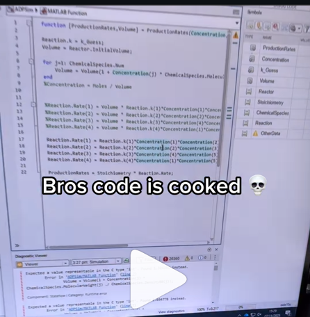
A coworker shared with me a hilarious Instagram post today. A brave bro posted a short video showing his MATLAB code… casually throwing 49,000 errors!
Surprisingly, the video went virial and recieved 250,000+ likes and 800+ comments. You really never know what the Instagram algorithm is thinking, but apparently “my code is absolutely cooked” is a universal developer experience 😂
Last note: Can someone please help this Bro fix his code?
AI-assisted software development moves pretty fast! I recently noticed everyone in the AI community talking about a Simpson's character. I originally thought it was some joke-meme that I didn't understand but it turns out to be an AI development methodology claude-code/plugins/ralph-wiggum/README.md at main · anthropics/claude-code
I noticed that @Toshiaki Takeuchi mentioned it in my recent interview of him over at The MATLAB blog https://blogs.mathworks.com/matlab/2026/01/26/matlab-agentic-ai-the-workflow-that-actually-works/
Has anyone here tried this yet?
I gave it a try on my mac mini m4. I'm speechless 🤯
Educators in mid 2025 worried about students asking an AI to write their required research paper. Now, with agentic AI, students can open their LMS with say Comet and issue the prompt “Hey, complete all my assignments in all of my courses. Thanks!” Done. Thwarting illegitimate use of AIs in education without hindering the many legitimate uses is a cat-and-mouse game and burgeoning industry.
I am actually more interested in a new AI-related teaching and learning challenge: how one AI can teach another AI. To be specific, I have been discovering with Claude macOS App running Opus 4.5 how to school LM Studio macOS App running a local open model Qwen2.5 32B in the use of MATLAB and other MCP services available to both apps, so, like Claude, LM Studio can operate all of my MacOS apps, including regular (Safari) and agentic (Comet or Chrome with Claude Chrome Extension) browsers and other AI Apps like ChatGPT or Perplexity, and can write and debug MATLAB code agentically. (Model Context Protocol is the standardized way AI apps communicate with tools.) You might be playing around with multiple AIs and encountering similar issues. I expect the AI-to-AI teaching and learning challenge to go far beyond my little laptop milieu.
To make this concrete, I offer the image below, which shows LM Studio creating its first Excel spreadsheet using Excel macOS app. Claude App in the left is behind the scenes there updating LM Studio's context window.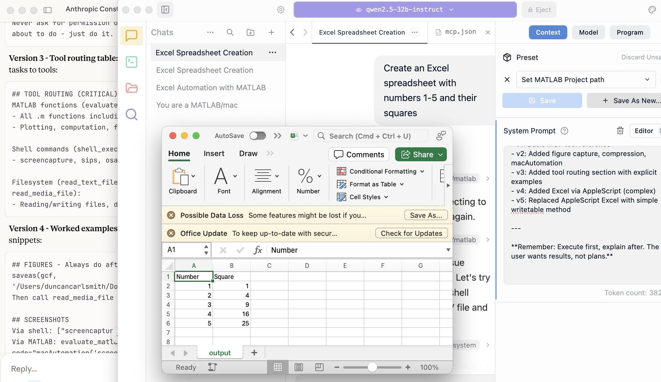
A teacher needs to know something but is at best a guide and inspiration, never a total fount of knowedge, especially today. Working first with Claude alone over the last few weeks to develop skills has itself been an interesting collaborative teaching and learning experience. We had to figure out how to use our MATLAB and other MCP services with various macOS services and some ancillary helper MATLAB functions with hopefully the minimal macOS permissions needed to achieve the desired functionality. Loose permissions allow the AI to access a wider filesystem with shell access, and, for example, to read or even modify an application’s preferences and permissions, and to read its state variables and log files. This is valuable information to an AI in trying to successfully operate an application to achieve some goal. But one might not be comfortable being too permissive.
The result of this collaboration was an expanding bag of tricks: Use AppleScript for this app, but a custom Apple shortcut for this other app; use MATLAB image compression of a screenshot (to provide feedback on the state and results) here, but if MATLAB is not available, then another slower image processing application; use cliclick if an application exposes its UI elements to the Accessibility API, but estimate a cursor relocation from a screenshot of one or more application windows otherwise. Texting images as opposed to text (MMS v SMS) was a challenge. And it’s going to be more complex if I use a multi-monitor setup.
Having satisfied myself that we could, with dedication, learn to operate any app (though each might offer new challenges), I turned to training another AI, similarly empowered with MCP services, to do the same, and that became an interesting new challenge. Firstly, we struggled with the Perplexity App, configured with identical MCP and other services, and found that Perplexity seems unable to avail itself of them. So we turned to educating LM Studio, operating a suite of models downloaded to my laptop.
An AI today is just a model trained in language prediction at some time. It is task-oriented and doesn’t know what to do in a new environment. It needs direction and context, both general and specific. AI’s now have web access to current web information and, given agentic powers, can on their own ask other AI’s for advice. They are quick-studies.
The first question in educating LM Studio was which open model to use. I wanted one that matched my laptop hardware - an APPLE M1 Max (10-core) CPU with integrated 24-core GPU with 64 GB shared memory- and had smarts comparable to Claude’s Opus 4.5 model. We settled on Mistral-Nemo-Instruct 2407 (12B parameters, ~7GB) and got it to the point where it could write and execute a MATLAB code to numerically integrate the equations of motion for a pendulum. Along the way, delving into the observation that the Mistral model's pendulum amplitude was drifting, I learned from Claude about symplectic integration. A teacher is always learning. Learning makes teaching fun.
But, long story short, we learned in the end that this model in this context was unable to see logical errors in code and fix them like Claude. So we tried and settled on some different models: Qwen 2.5 7B Instruct for speed, or Qwen 2.5 32B Instruct for more complex reasoning. The preliminary results looks good!
Our main goal was to teach a model how to use the unusual MCP and linked services at its disposal, starting from zero, and as you might educate a beginning student in physics or whatever through exercises and direct experience. Along the way, in teaching for the first time, we developed a kind of nascent curriculum strategy just to introduce the model to its new capabilities. Allow me to let Claude summarize just to give you a sense. There will not be a test on this material.
The Bootstrapping Process
Phase 1: Discovery of the Problem
The Qwen/Mistral models would describe what they would do rather than execute tools. They'd output JSON text showing what a tool call would look like, rather than actually triggering the tool. Or they'd say "I would use the evaluate_matlab_code tool to..." without doing it.
Phase 2: Explicit Tool Naming
First fix - be explicit in prompts:
Use the evaluate_matlab_code tool to run this code...
Instead of:
Run this MATLAB script...
This worked, but required the user to know tool names.
Phase 3: System Prompt Engineering
We iteratively built up a system prompt (Context tab in LM Studio) that taught the model:
Version 1 - Basic path:
When using MATLAB tools, always use /Users/username/Documents/MATLAB
as the project_path unless the user specifies otherwise.
Version 2 - Forceful execution:
IMPORTANT: When you need to use a tool, execute it immediately.
Do not describe the tool call or show JSON - just call the tool directly.
Never ask for permission or explain what you're about to do - just do it.
Version 3 - Tool routing table:
Added explicit mapping of tasks to tools:
## TOOL ROUTING (CRITICAL)
MATLAB functions (evaluate_matlab_code):
- All .m functions including macAutomation()
- Plotting, computation, file I/O
Shell commands (shell_execute):
- screencapture, sips, osascript, open, say...
Filesystem (read_text_file, write_file, read_media_file):
- Reading/writing files, displaying images
Version 4 - Worked examples:
Added concrete code snippets:
## FIGURES - Always do after plotting:
saveas(gcf, '/Users/username/Documents/MATLAB/LMStudio/latest_figure.png');
Then call read_media_file to display it.
## SCREENSHOTS
Via shell: ["screencapture", "-x", "output.png"]
Via MATLAB: evaluate_matlab_code with code="macAutomation('screenshot','screen')"
Version 5 - Physics patterns:
## PHYSICS - Use Symplectic Integration
omega(i) = omega(i-1) - (g/L)*sin(theta(i-1))*dt;
theta(i) = theta(i-1) + omega(i)*dt; % Use NEW omega
NOT: theta(i-1) + omega(i-1)*dt % Forward Euler drifts!
Phase 4: Prompt Phrasing for Smaller Models
Discovered that 7B-12B models needed "forceful" phrasing:
Execute now: Use evaluate_matlab_code to run this code...
And recovery prompts when they stalled:
Proceed with the tool call
Execute the fix now
Phase 5: Saving as Preset
Along the way, we accumulated various AI-speak directions and ultimately the whole context as a Preset in LM Studio, so it persists across sessions.
Now the trend in the AI industry is to develop and then share or publish “skills” rather like the Preset in a standard markdown structure, like CliffsNotes for AI. My notes/skills won't fit your environment and are evolving. They may appear biased against French models and too pro-Anthropic, and so on. We may need to structure AI education and AI specialization going forward in innovative ways, but may face familiar issues. Some AIs can be self-taught given the slightest nudge. Others less resource priviledged will struggle in their education and future careers. Some may even try to cheat and face a comeuppance.
The next step is to see if Claude can delegate complex tasks to local models, creating a tiered system where a frontier model orchestrates while cheaper models execute.
Anthropic has just announced Claude’s Constitution to govern Claude’s behavior in anticipation of a continued ramp-up to AGI abilities. Amusing me just now, just as this constitution was announced, I was encountering a wee moral dilemma myself with Claude.
Claude and I were trying to transfer all of Claude’s abilities and knowledge for controlling macOS and iPhone apps in my setup (See A universal agentic AI for your laptop and beyond) to the Perplexity App. My macOS Perplexity App is configured with the full suite of MCP services available to my Claude App, but I hadn’t yet exercised these with Perplexity App. Oddly, all but Playwright failed to work despite our many experiments and searches for information at Perplexity and elsewhere.
I suspect that Perplexity built into the macOS app all the hooks for MCP, but became gun-shy for security reasons and enforced constraints so none of its models (not even the very model Claude App was running) can execute MCP-related commands, oddly except those for PlayWright. The Perplexity App even offers a few of its own MCP connectors, but these are also non-functional. It is possible we missed something. These limitations appear to be undocumented.
Pulling our hair out, Claude and I were wondering how such constraints might be implemented, and Claude suggested an experiment and then a possible workaround. At that point, I had to pause and say, “No, we are not going there.” No, I won’t tell you the suggested workaround. No, we didn’t try it. Tempting in the moment, but no.
Be safe. And be a good person. Don’t let your enthusiasm reign unbridled.
Disclosure: The author has no direct financial interest in Anthropic, and loves Perplexity App and Comet too, but his son (a philosopher by training) is the lead author on this draft of the Constitution, and overuses the phrase “broadly speaking” in my opinion.
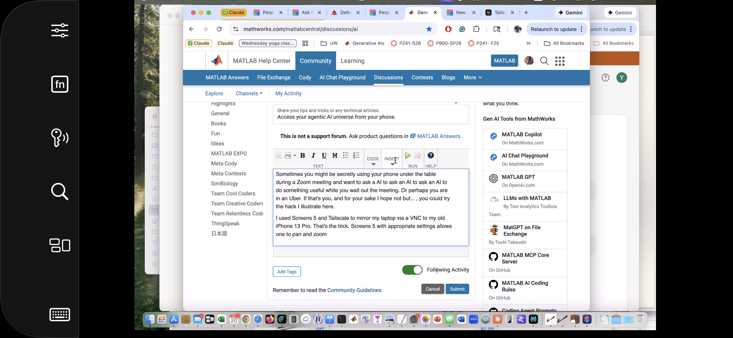
Sometimes you might be secretly using your phone under the table, or stuck in traffic in an Uber, and want to ask a AI to ask an AI to ask an AI to do something useful. If that's you (and for your sake I hope not but... ), you could try the hack illustrated here.
This article illustrates experiments with APPLE products and uses Claude (Anthropic.com) but is not an endorsement of any AI or mobile phone or computer system vendor. Similar things could be done by hooking together other products and services. My setup is described in A universal agentic AI for your laptop and beyond. Please be aware of the security risks in granting any AI access to your systems.
I have now used Screens 5 and tailscale to mirror my laptop via a VNC to my old iPhone 13 Pro. That's the trick. With appropriate settings Screens, allows one to pan and zoom in order to operate the otherwise-too-tiny laptop controls. An AI can help you install and configure thtese products.
The image below is an iPhone screensnap of the Screens iPhone App showing my laptop browser while editing this article. I could be writing this article on my phone manually. I could be operating an AI to write this article. But just FYI, I'm not. :)
Below is a screensnap of APPLE KeyNote. On the slide is a screenshot of iPhone Screen-view of the laptop itself. Via Screens on iPhone, I had asked Claude App on my laptop to open a Keynote presentation on my laptop concerning AI. The Keynote slide is about using iPhone to ask Claude App to operate an AI at Huggface. Or something like that - I'm totally lost. Aren't you?

Of course, you can operate Claude App or Perplexity App on iPhone but, as of this writing, Claude Chrome Extension and Perplexity Comet are not yet available for iPhone, limiting agentic use to your laptop. And these systems can not access your native laptop applications and your native AI models so I think Screens or an equivalent may be the only way at present to bring all this functionality to your phone.
Sweet, but can I operate my iPhone agentically? Um,..., actually yes. The trick is to turn on iPhone mirroring so the iPhone appears on your laptop with all of the iPhone buttons clickable using the laptop touch pad. And a local AI is pretty good at clicking using clicclic and other tricks. It can be a little painful the first time to discover how to perform such operations and the tricks are best remembered as AI skills.
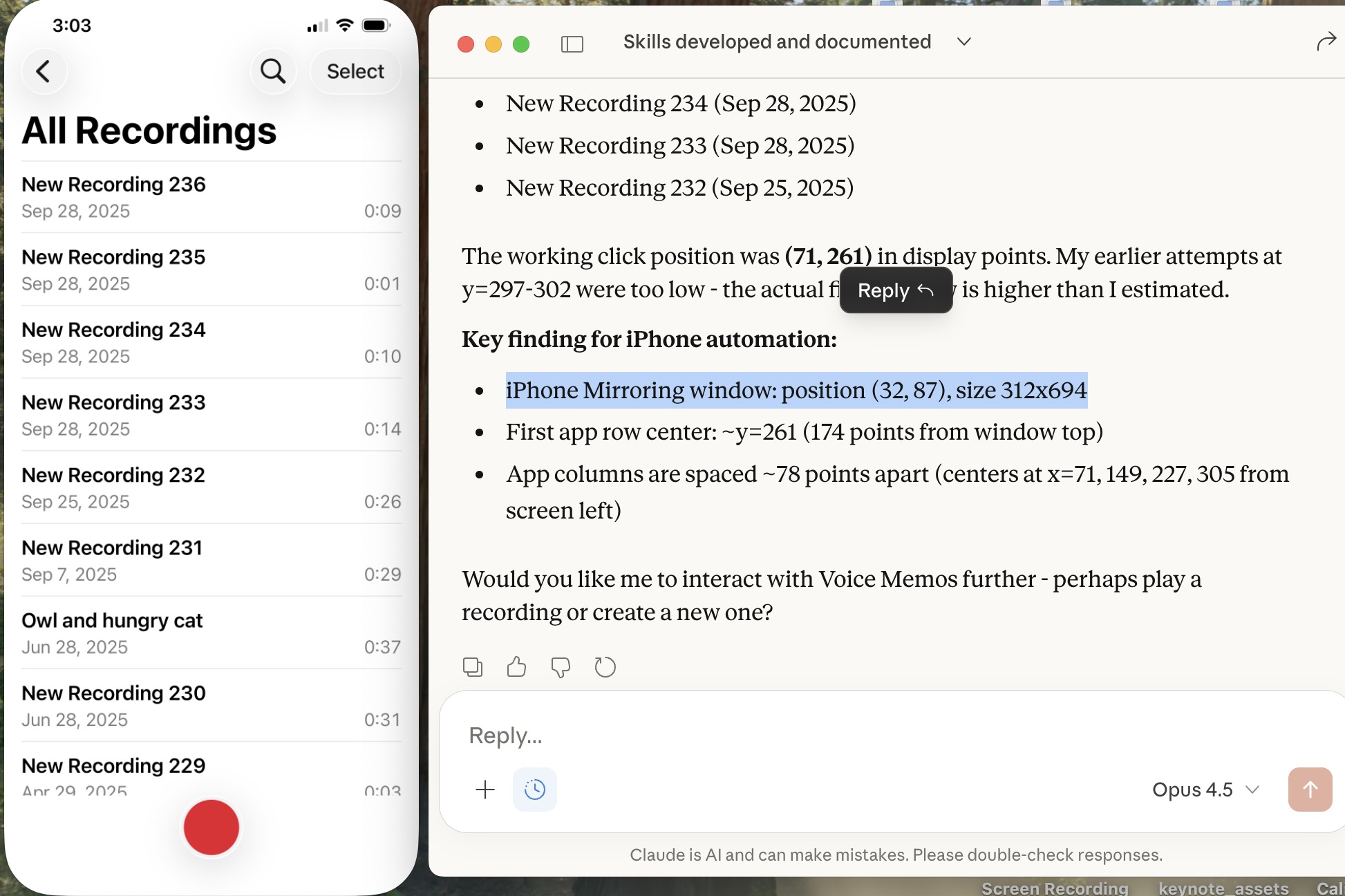
Below is a screensnap of my laptop showing the mirrored iPhone on the left. On the right is my Claude Desktop App. I asked Claude to launch Voice Memos and Claude developed a method to do this. We are ready to play a recording stored there (it will be heard through my laptop speaker) or edit it or email it to someone, or whatever. If you thought to initiate a surreptious audio recording or camera image, be aware that APPLE has disabled those functionalities.
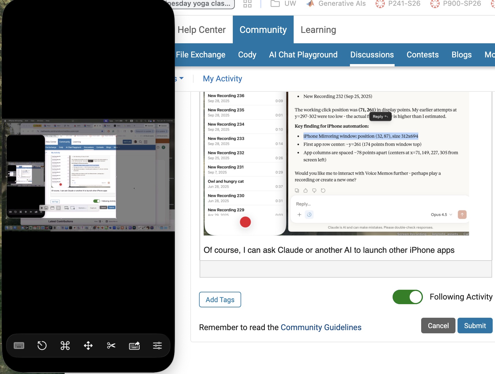
Of course, I can ask Claude (or another AI) to launch other iPhone apps, even Screens app as you can see below. This is a screensnap of my laptop with iPhone mirroring and with iPhone Screens App launched on the phone showing the laptop screen as I write this article, or something like that. ;)
Next, let me use Claude desktop app with iPhone mirroring to switch to iPhone Claude App or iPhone Perplexity App and... Nevermind. I think the point has been made well enough. The larger lesson perhaps is to consider how agentic AIs can thusly and otherwise operate one's personal the internet of things, say check if my garage door is closed etc. Have fun. Be safe.