eqn =
Results for
I have a skeleton and i want to find the start and end point of that skeleton. My skeleton is like an oval/donut where there is little gap between the start and end
Hello,
Now that the "Copilot+PC" (Windows ARM) laptops are rapidly increasing in market share (Microsoft Surface Laptop, Dell XPS 13, HP OmniBook X 14, and more), are there any plans to provide builds for Matlab on Windows arm64?
Since there are already Windows builds of Matlab, it shouldn't be too hard to compile for Windows arm64, as far as I know. But I am not famaliar with Matlab's codebase.
Please try to publish Windows arm64 builds soon so that Matlab can be much more usable on Windows on ARM as it will run natively instead of in emulation.
Thank you very much.
Attaching the Photoshop file if you want to modify the caption.
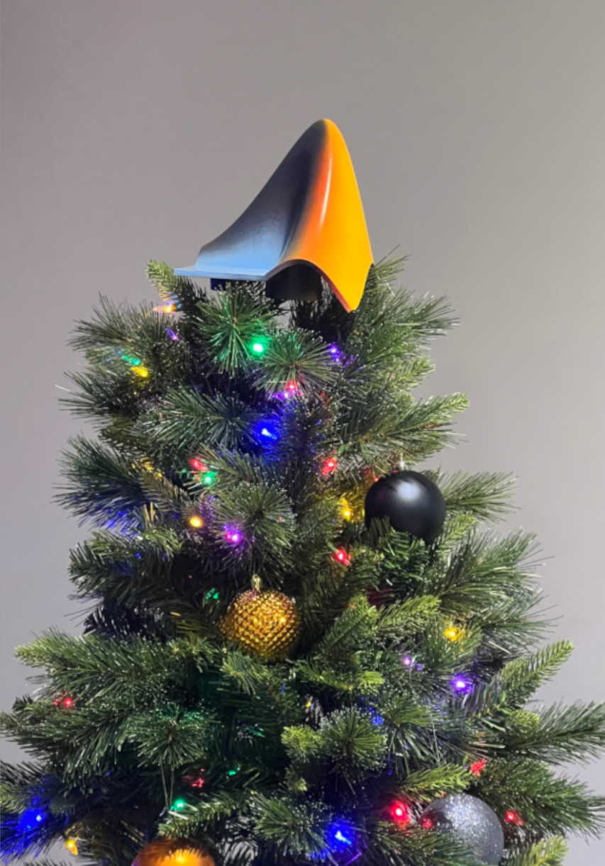
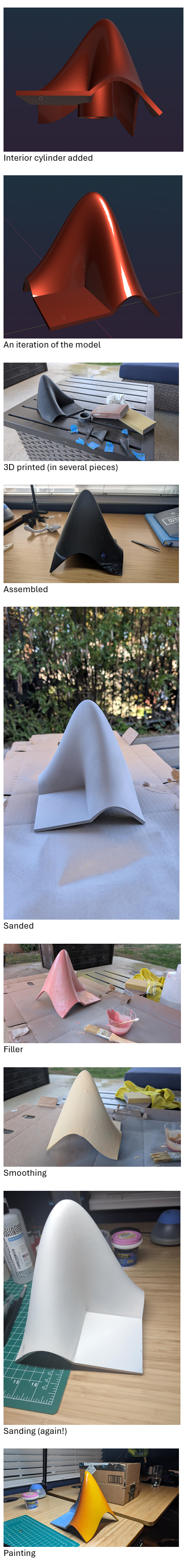
What better way to add a little holiday magic than the L-shaped membrane atop your evergreen? My colleagues output the shape and then added some thickness and an interior cylinder in Blender. Then, the shape was exported to STL and 3D printed (in several pieces). Then glued, sanded, primed, sanded again and painted. If you like, the STL file is attached. Thank you to https://blogs.mathworks.com/community/2013/06/20/paul-prints-the-l-shaped-membrane/ and a tip of the hat to MATLAB Ornament. Happy Holidays!
I have a problem with the movement of a pawn by two fields in its first move does anyone have a suggestion for a solution
function chess_game()
% Funkcja główna inicjalizująca grę w szachy
% Inicjalizacja stanu gry
gameState = struct();
gameState.board = initialize_board();
gameState.currentPlayer = 'white';
gameState.selectedPiece = [];
% Utworzenie GUI
fig = figure('Name', 'Gra w Szachy', 'NumberTitle', 'off', 'MenuBar', 'none', 'UserData', gameState);
ax = axes('Parent', fig, 'Position', [0 0 1 1], 'XTick', [], 'YTick', []);
axis(ax, [0 8 0 8]);
hold on;
% Wyświetlenie planszy
draw_board(ax, gameState.board);
% Obsługa kliknięcia myszy
set(fig, 'WindowButtonDownFcn', @(src, event)on_click(ax, src));
end
function board = initialize_board()
% Inicjalizuje planszę z ustawieniem początkowym figur
board = {
'R', 'N', 'B', 'Q', 'K', 'B', 'N', 'R';
'P', 'P', 'P', 'P', 'P', 'P', 'P', 'P';
'', '', '', '', '', '', '', '';
'', '', '', '', '', '', '', '';
'', '', '', '', '', '', '', '';
'', '', '', '', '', '', '', '';
'p', 'p', 'p', 'p', 'p', 'p', 'p', 'p';
'r', 'n', 'b', 'q', 'k', 'b', 'n', 'r';
};
end
function draw_board(~, board)
% Rysuje szachownicę i figury
colors = [1 1 1; 0.8 0.8 0.8];
for row = 1:8
for col = 1:8
% Rysowanie pól
rectColor = colors(mod(row + col, 2) + 1, :);
rectangle('Position', [col-1, 8-row, 1, 1], 'FaceColor', rectColor, 'EdgeColor', 'k');
% Rysowanie figur
piece = board{row, col};
if ~isempty(piece)
text(col-0.5, 8-row+0.5, piece, 'HorizontalAlignment', 'center', ...
'FontSize', 20, 'FontWeight', 'bold');
end
end
end
end
function on_click(ax, fig)
% Funkcja obsługująca kliknięcia myszy
pos = get(ax, 'CurrentPoint');
x = floor(pos(1,1)) + 1; % Zaokrąglij współrzędne w poziomie i dopasuj do indeksów
y = 8 - floor(pos(1,2)); % Dopasuj współrzędne w pionie (odwrócenie osi Y)
% Pobranie stanu gry z figury
gameState = get(fig, 'UserData');
if x >= 1 && x <= 8 && y >= 1 && y <= 8
disp(['Kliknięto na pole: (', num2str(x), ', ', num2str(y), ')']);
if isempty(gameState.selectedPiece)
% Wybór figury
piece = gameState.board{y, x};
if ~isempty(piece)
if (strcmp(gameState.currentPlayer, 'white') && any(ismember(piece, 'RNBQKP'))) || ...
(strcmp(gameState.currentPlayer, 'black') && any(ismember(piece, 'rnbqkp')))
gameState.selectedPiece = [y, x];
disp(['Wybrano figurę: ', piece, ' na pozycji (', num2str(x), ', ', num2str(y), ')']);
else
disp('Nie możesz wybrać tej figury.');
end
else
disp('Nie wybrano figury.');
end
else
% Sprawdzenie, czy kliknięto ponownie na wybraną figurę
if isequal(gameState.selectedPiece, [y, x])
disp('Anulowano wybór figury.');
gameState.selectedPiece = [];
else
% Ruch figury
[sy, sx] = deal(gameState.selectedPiece(1), gameState.selectedPiece(2));
piece = gameState.board{sy, sx};
if is_valid_move(gameState.board, piece, [sy, sx], [y, x], gameState.currentPlayer)
% Wykonanie ruchu
gameState.board{sy, sx} = ''; % Usuwamy figurę z poprzedniego pola
gameState.board{y, x} = piece; % Umieszczamy figurę na nowym polu
gameState.selectedPiece = [];
% Przełącz gracza
gameState.currentPlayer = switch_player(gameState.currentPlayer);
% Odśwież planszę
cla(ax);
draw_board(ax, gameState.board);
else
disp('Ruch niezgodny z zasadami.');
end
end
end
% Zaktualizowanie stanu gry w figurze
set(fig, 'UserData', gameState);
end
end
function valid = is_valid_move(board, piece, from, to, currentPlayer)
% Funkcja sprawdzająca, czy ruch jest poprawny
[sy, sx] = deal(from(1), from(2));
[dy, dx] = deal(to(1), to(2));
dy_diff = dy - sy;
dx_diff = abs(dx - sx);
targetPiece = board{dy, dx};
% Sprawdzenie, czy ruch jest w granicach planszy
if dx < 1 || dx > 8 || dy < 1 || dy > 8
valid = false;
return;
end
% Nie można zbijać swoich figur
if ~isempty(targetPiece) && ...
((strcmp(currentPlayer, 'white') && ismember(targetPiece, 'RNBQKP')) || ...
(strcmp(currentPlayer, 'black') && ismember(targetPiece, 'rnbqkp')))
valid = false;
return;
end
% Zasady ruchu dla każdej figury
switch lower(piece)
case 'p' % Pion
direction = strcmp(currentPlayer, 'white') * 2 - 1; % 1 dla białych, -1 dla czarnych
startRow = strcmp(currentPlayer, 'white') * 2 + 1; % Rząd startowy dla białych i czarnych
if isempty(targetPiece)
% Ruch o jedno pole do przodu
if dy_diff == direction && dx_diff == 0
valid = true;
% Ruch o dwa pola do przodu z pozycji startowej
elseif dy_diff == 2 * direction && dx_diff == 0 && sy == startRow
if isempty(board{sy + direction, sx}) && isempty(board{dy, dx})
valid = true;
else
valid = false;
end
else
valid = false;
end
else
% Zbijanie na ukos
valid = (dx_diff == 1) && (dy_diff == direction);
end
case 'r' % Wieża
valid = (dx_diff == 0 || dy_diff == 0) && path_is_clear(board, from, to);
case 'n' % Skoczek
valid = (dx_diff == 2 && abs(dy_diff) == 1) || (dx_diff == 1 && abs(dy_diff) == 2);
case 'b' % Goniec
valid = (dx_diff == abs(dy_diff)) && path_is_clear(board, from, to);
case 'q' % Hetman
valid = ((dx_diff == 0 || dy_diff == 0) || (dx_diff == abs(dy_diff))) && path_is_clear(board, from, to);
case 'k' % Król
valid = max(abs(dx_diff), abs(dy_diff)) == 1;
otherwise
valid = false;
end
end
function clear = path_is_clear(board, from, to)
% Sprawdza, czy ścieżka między polami jest wolna od innych figur
[sy, sx] = deal(from(1), from(2));
[dy, dx] = deal(to(1), to(2));
stepY = sign(dy - sy);
stepX = sign(dx - sx);
y = sy + stepY;
x = sx + stepX;
while y ~= dy || x ~= dx
if ~isempty(board{y, x})
clear = false;
return;
end
y = y + stepY;
x = x + stepX;
end
clear = true;
end
function nextPlayer = switch_player(currentPlayer)
% Przełącza aktywnego gracza
if strcmp(currentPlayer, 'white')
nextPlayer = 'black';
else
nextPlayer = 'white';
end
end
Speaking as someone with 31+ years of experience developing and using imshow, I want to advocate for retiring and replacing it.
The function imshow has behaviors and defaults that were appropriate for the MATLAB and computer monitors of the 1990s, but which are not the best choice for most image display situations in today's MATLAB. Also, the 31 years have not been kind to the imshow code base. It is a glitchy, hard-to-maintain monster.
My new File Exchange function, imview, illustrates the kind of changes that I think should be made. The function imview is a much better MATLAB graphics citizen and produces higher quality image display by default, and it dispenses with the whole fraught business of trying to resize the containing figure. Although this is an initial release that does not yet support all the useful options that imshow does, it does enough that I am prepared to stop using imshow in my own work.
The Image Processing Toolbox team has just introduced in R2024b a new image viewer called imageshow, but that image viewer is created in a special-purpose window. It does not satisfy the need for an image display function that works well with the axes and figure objects of the traditional MATLAB graphics system.
I have published a blog post today that describes all this in more detail. I'd be interested to hear what other people think.
Note: Yes, I know there is an Image Processing Toolbox function called imview. That one is a stub for an old toolbox capability that was removed something like 15+ years ago. The only thing the toolbox imview function does now is call error. I have just submitted a support request to MathWorks to remove this old stub.
The int function in the Symbolic Toolbox has a hold/release functionality wherein the expression can be held to delay evaluation
syms x I
eqn = I == int(x,x,'Hold',true)
which allows one to show the integral, and then use release to show the result
release(eqn)
Maybe it would be nice to be able to hold/release any symbolic expression to delay the engine from doing evaluations/simplifications that it typically does. For example:
x*(x+1)/x, sin(sym(pi)/3)

If I'm trying to show a sequence of steps to develop a result, maybe I want to explicitly keep the x/x in the first case and then say "now the x in the numerator and denominator cancel and the result is ..." followed by the release command to get the final result.
Perhaps held expressions could even be nested to show a sequence of results upon subsequent releases.
Held expressions might be subject to other limitations, like maybe they can't be fplotted.
Seems like such a capability might not be useful for problem solving, but might be useful for exposition, instruction, etc.
I want to build a neural network that takes a matrix A as input and outputs a matrix B such that a constant C=f(A,B)is maximized as much as possible.(The function f()is a custom complex computation function involving random values,probability density,matrix norms,and a series of other calculations).
I tried to directly use 1/f(A,B)or-f(A,B)as the loss function,but I encountered an error stating:"The value to be differentiated is not tracked.It must be a tracked real number dlarray scalar.Use dlgradient to track variables in the function called by dlfeval."I suspect this is likely because f(A,B)is not differentiable.
However,I've also seen people say that no matter what function it is,the dlgradient function can differentiate it.
So,I'm not sure whether it's because the function f()is too complex to be used as a loss function to calculate gradients,or if there's an issue with my code.
If I can't directly use its reciprocal or negative as the loss function,how should I go about training this neural network?Currently,I only know how to implement:providing target values and using functions like mse or huber as loss functions.


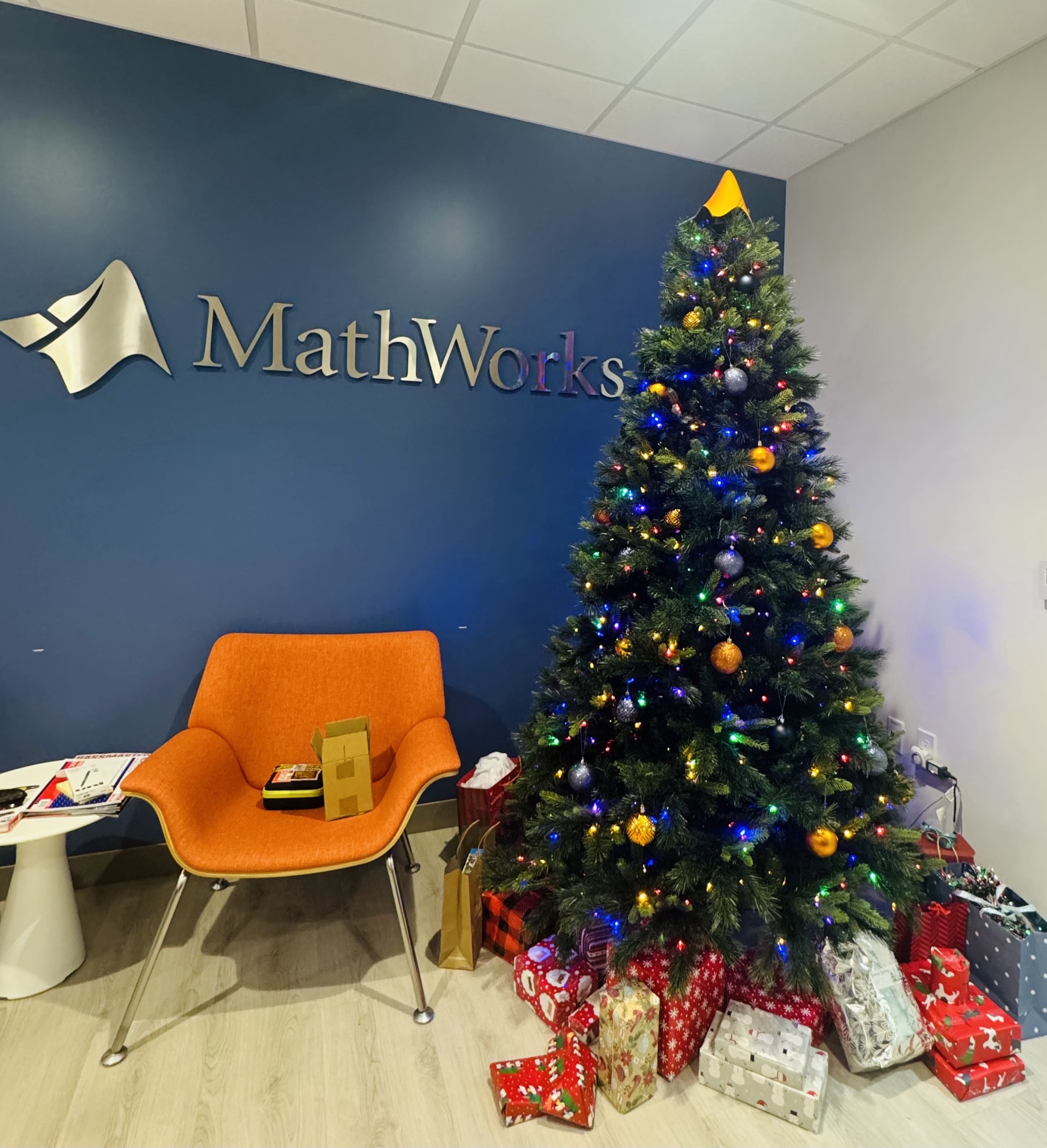
Christmas season is underway at my house:

(Sorry - the ornament is not available at the MathWorks Merch Shop -- I made it with a 3-D printer.)
We are thrilled to announce the grand prize winners of our MATLAB Shorts Mini Hack contest! This year, we invited the MATLAB Graphics and Charting team, the authors of the MATLAB functions used in every entry, to be our judges. After careful consideration, they have selected the top three winners:
Judge comments: Realism & detailed comments; wowed us with Manta Ray
2nd place – Jenny Bosten
Judge comments: Topical hacks : Auroras & Wind turbine; beautiful landscapes & nightscapes
3rd place - Vasilis Bellos
Judge comments: Nice algorithms & extra comments; can’t go wrong with Pumpkins
Judge comments: Impressive spring & cubes!
In addition, after validating the votes, we are pleased to announce the top 10 participants on the leaderboard:
Congratulations to all! Your creativity and skills have inspired many of us to explore and learn new skills, and make this contest a big success!
Dear MATLAB contest enthusiasts,
Welcome to the third installment of our interview series with top contest participants! This time we had the pleasure of talking to our all-time rock star – @Jenny Bosten. Every one of her entries is a masterpiece, demonstrating a deep understanding of the relationship between mathematics and aesthetics. Even Cleve Moler, the original author of MATLAB, is impressed and wrote in his blog: "Her code for Time Lapse of Lake View to the West shows she is also a wizard of coordinate systems and color maps."
you to read it to learn more about Jenny’s journey, her creative process, and her favorite entries.
Question: Who would you like to see featured in our next interview? Let us know your thoughts in the comments!
It would be nice to have a function to shade between two curves. This is a common question asked on Answers and there are some File Exchange entries on it but it's such a common thing to want to do I think there should be a built in function for it. I'm thinking of something like
plotsWithShading(x1, y1, 'r-', x2, y2, 'b-', 'ShadingColor', [.7, .5, .3], 'Opacity', 0.5);
So we can specify the coordinates of the two curves, and the shading color to be used, and its opacity, and it would shade the region between the two curves where the x ranges overlap. Other options should also be accepted, like line with, line style, markers or not, etc. Perhaps all those options could be put into a structure as fields, like
plotsWithShading(x1, y1, options1, x2, y2, options2, 'ShadingColor', [.7, .5, .3], 'Opacity', 0.5);
the shading options could also (optionally) be a structure. I know it can be done with a series of other functions like patch or fill, but it's kind of tricky and not obvious as we can see from the number of questions about how to do it.
Does anyone else think this would be a convenient function to add?
Over the past 4 weeks, 250+ creative short movies have been crafted. We had a lot of fun and, more importantly, learned new skills from each other! Now it’s time to announce week 4 winners.
Nature:
3D:
Seamless loop:
Holiday:
Fractal:
Congratulations! Each of you won your choice of a T-shirt, a hat, or a coffee mug. We will contact you after the contest ends.
Weekly Special Prizes
Thank you for sharing your tips & tricks with the community. These great technical articles will benefit community users for many years. You won a limited-edition pair of MATLAB Shorts!
In week 5, let’s take a moment to sit back, explore all of the interesting entries, and cast your votes. Reflect what you have learned or which entries you like most. Share anything in our Discussions area! There is still time to win our limited-edition MATLAB Shorts.
In the past two years, large language models have brought us significant changes, leading to the emergence of programming tools such as GitHub Copilot, Tabnine, Kite, CodeGPT, Replit, Cursor, and many others. Most of these tools support code writing by providing auto-completion, prompts, and suggestions, and they can be easily integrated with various IDEs.
As far as I know, aside from the MATLAB-VSCode/MatGPT plugin, MATLAB lacks such AI assistant plugins for its native MATLAB-Desktop, although it can leverage other third-party plugins for intelligent programming assistance. There is hope for a native tool of this kind to be built-in.
I know we have all been in that all-too-common situation of needing to inefficiently identify prime numbers using only a regular expression... and now Matt Parker from Standup Maths helpfully released a YouTube video entitled "How on Earth does ^.?$|^(..+?)\1+$ produce primes?" in which he explains a simple regular expression (aka Halloween incantation) which matches composite numbers:
Here is my first attempt using MATLAB and Matt Parker's example values:
fnh = @(n) isempty(regexp(repelem('*',n),'^.?$|^(..+?)\1+$','emptymatch'));
fnh(13)
fnh(15)
fnh(101)
fnh(1000)
Feel free to try/modify the incantation yourself. Happy Halloween!
We are thrilled to see the incredible short movies created during Week 3. The bar has been set exceptionally high! This week, we invited our Community Advisory Board (CAB) members to select winners. Here are their picks:
Mini Hack Winners - Week 3
Game:
Holidays:
Fractals:
Realism:
Great Remixes:
Seamless loop:
Fun:
Weekly Special Prizes
Thank you for sharing your tips & tricks with the community. You won a limited-edition MATLAB Shorts.
We still have plenty of MATLAB Shorts available, so be sure to create your posts before the contest ends. Don't miss out on the opportunity to showcase your creativity!
clc
clear
close all
% Load the dataset from a CSV file with headers
data = readtable('C:\Users\PMLS\Downloads\output_file.csv');
% Convert the table to a numeric array
dataArray = table2array(data);
% Normalize inputs and outputs using mapminmax
X = mapminmax(dataArray(:, 1:4)', 0, 1); % Normalize input features to [0, 1]
Y = mapminmax(dataArray(:, 5)', 0, 1); % Normalize target variable to [0, 1]
% Set display format to long for better precision
format long;
%rng(0); % Set random seed for reproducibility
% Create a simpler network with one hidden layer of 20 neurons
%net = feedforwardnet([40,70]);
net = feedforwardnet([70,40]);
% Change activation functions
net.layers{1}.transferFcn = 'poslin'; % ReLU
net.layers{2}.transferFcn = 'logsig'; % logsig
% Set the training function to Resilient Backpropagation
net.trainFcn = 'trainrp';
% Enable data division for validation and testing
net.divideFcn = 'divideblock';
net.divideParam.trainRatio = 0.8; % 70% training data
%net.divideParam.valRatio = 0.15; % 15% validation data
net.divideParam.testRatio = 0.2; % 15% testing data
% Custom training parameters
net.trainParam.epochs = 8000;
net.trainParam.goal = 0.0001;
net.trainParam.min_grad = 1e-6;
net.trainParam.max_fail = 2000;
net.trainParam.lr = 0.001; % Learning rate
net.trainParam.momentum = 0.9; % Momentum
%net.trainParam.batchSize = 10; % Example batch size
% Add regularization
net.performParam.regularization = 0.01; % Example L2 regularization
%Train the neural network
[net, tr] = train(net, X, Y);
% Predict and save results
predicted_ranges = net(X);
outputTable = array2table([X' Y' predicted_ranges'], ...
'VariableNames', {'w1', 'w2', 'w3', 'wpl', 'Actual_Range', 'Predicted_Range'});
writetable(outputTable, 'predicted_ranges_with_trainrp.xlsx');
% Calculate performance metrics
Y = Y'; % Transpose to match predicted output dimensions
predicted_ranges = predicted_ranges';
MAE = mean(abs(Y - predicted_ranges)); % Mean Absolute Error
MSE = mean((Y - predicted_ranges).^2); % Mean Squared Error
RMSE = sqrt(MSE); % Root Mean Square Error
R_squared = 1 - sum((Y - predicted_ranges).^2) / sum((Y - mean(Y)).^2); % R-squared
% Display the results in the command window
disp('Performance Metrics:');
disp(['Mean Absolute Error (MAE): ', num2str(MAE)]);
disp(['Mean Squared Error (MSE): ', num2str(MSE)]);
disp(['Root Mean Square Error (RMSE): ', num2str(RMSE)]);
disp(['R-squared (R^2): ', num2str(R_squared)]);
% Plot performance
plotperform(tr);
view(net);
% Plot the actual and predicted values as lines
figure;
plot(Y, 'b-', 'LineWidth', 1.5); % Plot actual values as a blue line
hold on;
plot(predicted_ranges, 'r--', 'LineWidth', 1.5); % Plot predicted values as a red dashed line
xlabel('Sample');
ylabel('Normalized Range');
legend('Actual Range', 'Predicted Range');
title('Comparison of Actual and Predicted Ranges');
grid on;