1922760350154212639070
Results for
How can we use roughness in an effective context to identify large primes? I can quickly think of quite a few examples where we might do so. Again, remember I will be looking for primes with not just hundreds of decimal digits, or even only a few thousand digits. The eventual target is higher than that. Forget about targets for now though, as this is a journey, and what matters in this journey is what we may learn along the way.
I think the most obvious way to employ roughness is in a search for twin primes. Though not yet proven, the twin prime conjecture:
If it is true, it tells us there are infinitely many twin prime pairs. A twin prime pair is two integers with a separation of 2, such that both of them are prime. We can find quite a few of them at first, as we have {3,5}, {5,7}, {11,13}, etc. But there is only ONE pair of integers with a spacing of 1, such that both of them are prime. That is the pair {2,3}. And since primes are less and less common as we go further out, possibly there are only a finite number of twins with a spacing of exactly 2? Anyway, while I'm fairly sure the twin prime conjecture will one day be shown to be true, it can still be interesting to search for larger and larger twin prime pairs. The largest such known pair at the moment is
2996863034895*2^1290000 +/- 1
This is a pair with 388342 decimal digits. And while seriously large, it is still in range of large integers we can work with in MATLAB, though certainly not in double precision. In my own personal work on my own computer, I've done prime testing on integers (in MATLAB) with considerably more than 100,000 decimal digits.
But, again you may ask, just how does roughness help us here? In fact, this application of roughness is not new with me. You might want to read about tools like NewPGen {https://t5k.org/programs/NewPGen/} which sieves out numbers known to be composite, before any direct tests for primality are performed.
Before we even try to talk about numbers with thousands or hundreds of thousands of decimal digits, look at 6=2*3. You might observe
isprime([-1,1] + 6)
shows that both 5 and 7 are prime. This should not be a surprise, but think about what happens, about why it generated a twin prime pair. 6 is divisible by both 2 and 3, so neither 5 or 7 can possibly be divisible by either small prime as they are one more or one less than a multiple of both 2 and 3. We can try this again, pushing the limits just a bit.
isprime([-1,1] + 2*3*5)
That is again interesting. 30=2*3*5 is evenly divisible by 2, 3, and 5. The result is both 29 and 31 are prime, because adding 1 or subtracting 1 from a multiple of 2, 3, or 5 will always result in a number that is not divisible by any of those small primes. The next larger prime after 5 is 7, but it cannot be a factor of 29 or 31, since it is greater than both sqrt(29) and sqrt(31).
We have quite efficiently found another twin prime pair. Can we take this a step further? 210=2*3*5*7 is the smallest such highly composite number that is divisible by all primes up to 7. Can we use the same trick once more?
isprime([-1,1] + 2*3*5*7)
And here the trick fails, because 209=11*19 is not in fact prime. However, can we use the large twin prime trick we saw before? Consider numbers of the form [-1,1]+a*210, where a is itself some small integer?
a = 2;
isprime([-1,1] + a*2*3*5*7)
I did not need to look far, only out to a=2, because both 419 and 421 are prime. You might argue we have formed a twin prime "factory", of sorts. Next, I'll go out as far as the product of all primes not exceeding 60. This is a number with 22 decimal digits, already too large to represent as a double, or even as uint64.
prod(sym(primes(60)))
a = find(all(isprime([-1;1] + prod(sym(primes(60)))*(1:100)),1))
That easily identifies 3 such twin prime pairs, each of which has roughly 23 decimal digits, each of which have the form a*1922760350154212639070+/-1. The twin prime factory is still working well. Going further out to integers with 37 decimal digits, we can easily find two more such pairs that employ the product of all primes not exceeding 100.
prod(sym(primes(100)))
a = find(all(isprime([-1;1] + prod(sym(primes(100)))*(1:100)),1))
This is in fact an efficient way of identifying large twin prime pairs, because it chooses a massively composite number as the product of many distinct small primes. Adding or subtracting 1 from such a number will result always in a rough number, not divisible by any of the primes employed. With a little more CPU time expended, now working with numbers with over 1000 decimal digits, I will claim this next pair forms a twin prime pair, and is the smallest such pair we can generate in this way from the product of the primes not exceeding 2500.
isprime(7826*prod(sym(primes(2500))) + [-1 1])
ans =
logical
1
Unfortunately, 1000 decimal digits is at or near the limit of what the sym/isprime tool can do for us. It does beg the question, asking if there are alternatives to the sym/isprime tool, as an isProbablePrime test, usually based on Miller-Rabin is often employed. But this is gist for yet another set of posts.
Anyway, I've done a search for primes of the form
a*prod(sym(primes(10000))) +/- 1
having gone out as far as a = 600000, with no success as of yet. (My estimate is I will find a pair by the time I get near 5e6 for a.) Anyway, if others can find a better way to search for large twin primes in MATLAB, or if you know of a larger twin prime pair of this extended form, feel free to chime in.
My next post shows how to use GCD in a very nice way to identify roughness, on a large scale.
What is a rough number? What can they be used for? Today I'll take you down a journey into the land of prime numbers (in MATLAB). But remember that a journey is not always about your destination, but about what you learn along the way. And so, while this will be all about primes, and specifically large primes, before we get there we need some background. That will start with rough numbers.
Rough numbers are what I would describe as wannabe primes. Almost primes, and even sometimes prime, but often not prime. They could've been prime, but may not quite make it to the top. (If you are thinking of Marlon Brando here, telling us he "could've been a contender", you are on the right track.)
Mathematically, we could call a number k-rough if it is evenly divisible by no prime smaller than k. (Some authors will use the term k-rough to denote a number where the smallest prime factor is GREATER than k. The difference here is a minor one, and inconsequential for my purposes.) And there are also smooth numbers, numerical antagonists to the rough ones, those numbers with only small prime factors. They are not relevant to the topic today, even though smooth numbers are terribly valuable tools in mathematics. Please forward my apologies to the smooth numbers.
Have you seen rough numbers in use before? Probably so, at least if you ever learned about the sieve of Eratosthenes for prime numbers, though probably the concept of roughness was never explicitly discussed at the time. The sieve is simple. Suppose you wanted a list of all primes less than 100? (Without using the primes function itself.)
% simple sieve of Eratosthenes
Nmax = 100;
N = true(1,Nmax); % A boolean vector which when done, will indicate primes
N(1) = false; % 1 is not a prime by definition
nextP = find(N,1,'first'); % the first prime is 2
while nextP <= sqrt(Nmax)
% flag multiples of nextP as not prime
N(nextP*nextP:nextP:end) = false;
% find the first element after nextP that remains true
nextP = nextP + find(N(nextP+1:end),1,'first');
end
primeList = find(N)
Indeed, that is the set of all 25 primes not exceeding 100. If you think about how the sieve worked, it first found 2 is prime. Then it discarded all integer multiples of 2. The first element after 2 that remains as true is 3. 3 is of course the second prime. At each pass through the loop, the true elements that remain correspond to numbers which are becoming more and more rough. By the time we have eliminated all multiples of 2, 3, 5, and finally 7, everything else that remains below 100 must be prime! The next prime on the list we would find is 11, but we have already removed all multiples of 11 that do not exceed 100, since 11^2=121. For example, 77 is 11*7, but we already removed it, because 77 is a multiple of 7.
Such a simple sieve to find primes is great for small primes. However is not remotely useful in terms of finding primes with many thousands or even millions of decimal digits. And that is where I want to go, eventually. So how might we use roughness in a useful way? You can think of roughness as a way to increase the relative density of primes. That is, all primes are rough numbers. In fact, they are maximally rough. But not all rough numbers are primes. We might think of roughness as a necessary, but not sufficient condition to be prime.
How many primes lie in the interval [1e6,2e6]?
numel(primes(2e6)) - numel(primes(1e6))
There are 70435 primes greater than 1e6, but less than 2e6. Given there are 1 million natural numbers in that set, roughly 7% of those numbers were prime. Next, how many 100-rough numbers lie in that same interval?
N = (1e6:2e6)';
roughInd = all(mod(N,primes(100)) > 0,2);
sum(roughInd)
That is, there are 120571 100-rough numbers in that interval, but all those 70435 primes form a subset of the 100-rough numbers. What does this tell us? Of the 1 million numbers in that interval, approximately 12% of them were 100-rough, but 58% of the rough set were prime.
The point being, if we can efficiently identify a number as being rough, then we can substantially increase the chance it is also prime. Roughness in this sense is a prime densifier. (Is that even a word? It is now.) If we can reduce the number of times we need to perform an explicit isprime test, that will gain greatly because a direct test for primality is often quite costly in CPU time, at least on really large numbers.
In my next post, I'll show some ways we can employ rough numbers to look for some large primes.
I am working on a project with tomosynthesis images of patients with breast cancer, in which I will use 3D CNNs. At the moment, I am selecting the slices where the cancer is visible, and my file format is DICOM. To use 3D CNNs, should I save the selected slices in a new single DICOM file, or should I save each slice in a separate file? What is the best format to use as input for my 3D CNN?
Additionally, to save the selected slices, which DICOM file metadata should I modify? I am modifying only the SOPInstanceUID and the PixelData.
When will the Mathlab issue about licence be resolved
Do you boast about the energy savings you racking up by using dark mode while stashing your energy bill savings away for an exotic vacation🌴🥥? Well, hold onto your sun hats and flipflops!
A recent study presented at the 1st Internaltional Workshop on Low Carbon Computing suggests that you may be burning more ⚡energy⚡ with your slick dark displays 💻[1].
In a 2x2 factorial design, ten participants viewed a webpage in dark and light modes in both dim and lit settings using an LCD monitor with 16 brightness levels.
- 80% of participants increased the monitor's brightness in dark mode [2]
- This occurred in both lit and dim rooms
- Dark mode did not reduce power draw but increasing monitor brightness did.
The color pixels in an LCD monitor still draw voltage when the screen is black, which is why the monitor looks gray when displaying a pure black background in a dark room. OLED monitors, on the other hand, are capable of turning off pixels that represent pure black and therefore have the potential to save energy with dark mode. A 2021 Purdue study estimates a 3%-9% energy savings with dark mode on OLED monitors using auto-brightness [3]. However, outside of gaming, OLED monitors have a very small market share and still account for less than 25% within the gaming world.
Any MATLAB users out there with OLED monitors? How are you going to spend your mad cash savings when you start using MATLAB's upcoming dark theme?
- BBC study: https://www.sicsa.ac.uk/wp-content/uploads/2024/11/LOCO2024_paper_12.pdf
- BBC blog article https://www.bbc.co.uk/rd/articles/2025-01-sustainability-web-energy-consumption
- 2021 Purdue https://dl.acm.org/doi/abs/10.1145/3458864.3467682
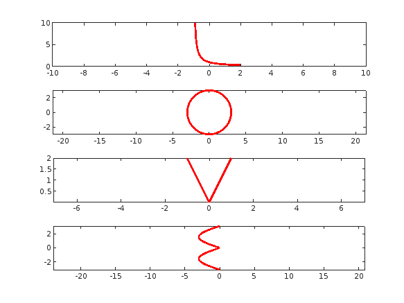
tiledlayout(4,1);
% Plot "L" (y = 1/(x+1), for x > -1)
x = linspace(-0.9, 2, 100); % Avoid x = -1 (undefined)
y =1 ./ (x+1) ;
nexttile;
plot(x, y, 'r', 'LineWidth', 2);
xlim([-10,10])
% Plot "O" (x^2 + y^2 = 9)
theta = linspace(0, 2*pi, 100);
x = 3 * cos(theta);
y = 3 * sin(theta);
nexttile;
plot(x, y, 'r', 'LineWidth', 2);
axis equal;
% Plot "V" (y = -2|x|)
x = linspace(-1, 1, 100);
y = 2 * abs(x);
nexttile;
plot(x, y, 'r', 'LineWidth', 2);
axis equal;
% Plot "E" (x = -3 |sin(y)|)
y = linspace(-pi, pi, 100);
x = -3 * abs(sin(y));
nexttile;
plot(x, y, 'r', 'LineWidth', 2);
axis equal;
syms p
f=2-ellipticK(p)
x0=0.1
a=fzero(f,x0)
I've been trying this problem a lot of time and i don't understand why my solution doesnt't work.
In 4 tests i get the error Assertion failed but when i run the code myself i get the diag and antidiag correctly.
function [diag_elements, antidg_elements] = your_fcn_name(x)
[m, n] = size(x);
% Inicializar los vectores de la diagonal y la anti-diagonal
diag_elements = zeros(1, min(m, n));
antidg_elements = zeros(1, min(m, n));
% Extraer los elementos de la diagonal
for i = 1:min(m, n)
diag_elements(i) = x(i, i);
end
% Extraer los elementos de la anti-diagonal
for i = 1:min(m, n)
antidg_elements(i) = x(m-i+1, i);
end
end
How do I make and export a brushed area from a figure
Hi all,
I'm working on quite some time to improve the code which I've written for better visualization of A0 mode. In my code everything looks good even I'm able to track the properties of the wave like out-of-plane and in-plane displacement but it is only evident and observable only at the extreme edges of the x (defined window). I'm attaching my code below. Any idea will be greatly appreciated. I'm also attaching the link of reference video which I'm trying to achieve or atleast anything close to it.
"freq = 2.5; %% KHz
Cpasym = 2.8953; %%phase velocity
d = 1; %% thickness of AL plate
Cl = 6.350; %% longitudnal velocity in the Al
Ct = 3.130; %% transverse velocity in the AL
zrange = -0.5:0.01:0.5;
shape = zeros(length(zrange),3);
for i = 1:length(zrange)
z = zrange(i);
shape(i,1) = z;
%% Mode shape in plane
Uasym = (2*pi*freq/Cpasym)*((sinh(sqrt(1/Cpasym^2-1/Cl^2)*2*pi*freq*z)/cosh(sqrt(1/Cpasym^2-1/Cl^2)*2*pi*freq*0.5*d))-(2*((2*pi*freq)^2*(1/Cpasym^2-1/Cl^2)^0.5*(1/Cpasym^2-1/Ct^2)^0.5)/((2/Cpasym^2-1/Ct^2)*(2*pi*freq)^2))*(sinh(sqrt(1/Cpasym^2-1/Ct^2)*2*pi*freq*z)/cosh(sqrt(1/Cpasym^2-1/Ct^2)*2*pi*freq*0.5*d)));
%% Mode shape out of plane
Wasym = (sqrt(1/Cpasym^2-1/Cl^2)*2*pi*freq)*((cosh(sqrt(1/Cpasym^2-1/Cl^2)*2*pi*freq*z)/cosh(sqrt(1/Cpasym^2-1/Cl^2)*2*pi*freq*0.5*d))-(2*(2*pi*freq/Cpasym)^2/((2/Cpasym^2-1/Ct^2)*(2*pi*freq)^2))*(cosh(sqrt(1/Cpasym^2-1/Ct^2)*2*pi*freq*z)/cosh(sqrt(1/Cpasym^2-1/Ct^2)*2*pi*freq*0.5*d)));
shape(i,2) = real(Uasym);
shape(i,3) = real(Wasym);
end
%% Normalizing the Mode shape
shape(:,2) = shape(:,2)/max(abs(shape(:,2)));
shape(:,3) = shape(:,3)/max(abs(shape(:,3)));
tvec = 0:0.01:10;
xvec = 0:0.01:9.5;
[X, Z] = meshgrid(xvec, zrange);
UAsym3D = zeros(length(zrange),length(xvec), length(tvec));
WAsym3D = zeros(length(zrange),length(xvec), length(tvec));
%% propogation governing equation
for i = 1:length(tvec)
for k = 1:length(xvec)
%for j = 1:length(zrange)
Ux = shape(:,2).*sin((2*pi*freq/Cpasym)*xvec(k)-(2*pi*freq*tvec(i)));
UAsym3D(:,k,i) = Ux;
Wz = shape(:,3).*cos((2*pi*freq/Cpasym)*xvec(k)-(2*pi*freq*tvec(i)));
WAsym3D(:,k,i) = Wz;
%end
end
end
% Normalize to [-1, 1]
UAsym3DN = UAsym3D / (max(abs(UAsym3D(:))));
WAsym3DN = WAsym3D / (max(abs(WAsym3D(:))));
% Create a VideoWriter object
videoFile = 'wave_motionAsym.avi'; % Output file name
writerObj = VideoWriter(videoFile , 'Motion JPEG AVI');
writerObj.FrameRate = 7; % Frames per second
open(writerObj);
hFig = figure('units','normalized','outerposition',[0 0 1 1]);
axis tight manual;
set(gca, 'NextPlot', 'replacechildren');
xlabel('x');
ylabel('z');
title('Resultant Displacement Anti-symmetric(A0) mode');
colormap(jet);
numTimeSteps = size(UAsym3DN, 3);
frames(numTimeSteps) = struct('cdata',[],'colormap',[]);
% Loop through each time step and create frames
for t = 1:size(UAsym3DN, 3)
% Get displacement at current time step
X_new = X + UAsym3DN(:,:, t); % Extract displacement at time t
Z_new = Z+ WAsym3DN(:,:, t); % Extract displacement at time t
scatter(X_new(:), Z_new(:), 5, 'filled');
%quiver(X(:), Z(:), Usym3DN(:,:, t),Wsym3DN(:,:, t), 'k','LineWidth',1);
xlabel('x'); ylabel('z');
axis([min(xvec)-1 max(xvec)+1 min(zrange)-1 max(zrange)+1]);
axis equal;
grid on;
drawnow;
pause(0.002);
frame = getframe(gcf);
frames(t) = frame;
writeVideo(writerObj, frame);
end
% Close the VideoWriter object
close(writerObj);
disp(['Movie saved as ', videoFile]);
implay('wave_motionAsym.avi');"
On 27th February María Elena Gavilán Alfonso and I will be giving an online seminar that has been a while in the making. We'll be covering MATLAB with Jupyter, Visual Studio Code, Python, Git and GitHub, how to make your MATLAB projects available to the world (no installation required!) and much much more.
Sign up (it's free!) at MATLAB Without Borders: Connecting your Projects with Python and other Open-Source Tools - MATLAB & Simulink

Hi Engineers,
I need your help to solve this. I am doing Power Systems Simulation Onramp, in that Represent Power Systems Components, @ Task 5, i have completed all the task instructions as mentioned, but not getting the output, i tried several times. kinldy help or suggest
My full funtion name is function [Y,t] = C2(Y0, dt, T) I have a secondary function dYdt = f_rhs(Y)
x = Y(1);
y = Y(2);
dx_dt = y;
dy_dt = -x + (1 - x^2) .* y;
dYdt = [dx_dt; dy_dt];
end
I keep geting an error when ever I try and add f_rhs into the code for it to call back on - Unable to define function C2 because it has the same name as the file. Any sugesstions?
Of course
62.5%
I never tried
37.5%
16 votes
Hi Control Experts,
I am designing an LQR controller for a system with time delay. The time delay is likely to be an input delay, but there is no certainty.
I have modelled the system as a continuous-time state space system, and I modelled the time delay with Pade approximation.
- I used the pade function in MATLAB to get the Pade transfer function, then I convert into state-space. I augmented the Pade state-space matrices with the state-space matrices of my plant. Am I taking the correct approach?
- My Pade approximation is 2nd order, so my state-space system now have 2 additional states. If I use MATLAB lqr function to get the LQR matrix K, what should the weightings of the Pade states be? Should they be set to very low (because we do not care about set point tracking of Pade states) or very high?
- Can I get some resources (even university lecture materials) that show how to design LQR for systems with time delays modelled with Pade approximations?
Thank you!
So I have taken the 3D UAV obstacle avoidance example and implemeneted path planning using DDPG on it. My agent learns to take the shortest path by avoiding the obstacle but as soon as I define a reset function and spawning the location of the agent between 2 postions it fails to learn. The main issue is that during a single training it learns to reach the goal from one position and when it is spawned to another location it was trainined on it takes the same path as before. The training for a single position is trained in like 100 to 150 episodes whereas when I spawn to two locations it wont converge ever after 10000 episodes.
I'll share the training curve for the agent being spawned at two locations.( Episodes greater than equal to 150 represent that it has reached the goal in the shortest path)
Observation:
Lidar Ranges (40 total ranges with max range of 5)
distance to goal
derivative of distance to goal
(I also tried adding more things to my observation such as pitch,yaw,roll and etc but that ultimately made the agent unable to converge faster)
Actions:
Pitch and Roll( -pi/7 to pi/7)
Yaw (-pi to pi)
Reward Function
Pitch, Roll and Yaw have a very small penalty
Penalty for hitting Obstacle (Large)
Reaching Goal
if derivative of disatance to goal is less than 0 its absoulte value is given as reward with a gain( rewarding the agent to maximize it velocity in the direction of the Goal)
minor step penalty
Termination Criteria:
If hit obstacle
If reached goal
Create the agent options object
agentOptions = rlDDPGAgentOptions();
% specify the options
agentOptions.SampleTime = Ts; %sampling time of 0.025 and final time of 25
agentOptions.MiniBatchSize = 256;
agentOptions.ExperienceBufferLength = 1e6;
agentOptions.MaxMiniBatchPerEpoch = 200;
% optimizer options
agentOptions.ActorOptimizerOptions.LearnRate = 1e-3;
agentOptions.ActorOptimizerOptions.GradientThreshold = 1;
agentOptions.CriticOptimizerOptions.LearnRate = 1e-3;
agentOptions.CriticOptimizerOptions.GradientThreshold = 1;
% exploration options
agentOptions.NoiseOptions.StandardDeviation = 0.15;
agentOptions.NoiseOptions.MeanAttractionConstant = 0.15;
initOpts = rlAgentInitializationOptions(NumHiddenUnit=256);
UAVQuadrotor = rlDDPGAgent(obsInfo,actInfo,initOpts,agentOptions);
Check out the result of "emoji matrix" multiplication below.
- vector multiply vector:
a = ["😁","😁","😁"]
b = ["😂";
"😂"
"😂"]
c = a*b
d = b*a
- matrix multiply matrix:
matrix1 = [
"😀", "😃";
"😄", "😁"]
matrix2 = [
"😆", "😅";
"😂", "🤣"]
resutl = matrix1*matrix2
enjoy yourself!
Creating data visualizations
79%
Interpreting data visualizations
21%
28 votes
what is the new modification for matlab 2024 and 2023b version , some of my code is showing error?
2024a版本下的runtime进行complier程序封装后,封装后的程序怎么在win7系统上使用?会显示很多不兼容问题,需要配置很多dll文件,能不能在封装时候就解决这些问题。