ans =
Main Content
Results for
Inspired by the suggestion of Mr. Chen Lin (MathWorks), I am writing this post with a humble and friendly intent to share some fascinating insights and knowledge about the Schwarzschild radius. My entry, which is related to this post, is named: 'Into the Abyss - Schwarzschild Radius (a time lapse)'.
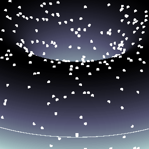
The Schwarzschild radius (or gravitational radius) defines the radius of the event horizon of a black hole, which is the boundary beyond which nothing, not even light, can escape the gravitational pull of the black hole. This concept comes from the Schwarzschild solution to Einstein’s field equations in general relativity. Black holes are regions of spacetime where gravitational collapse has caused matter to be concentrated within such a small volume that the escape velocity exceeds the speed of light.
This is a rudimentary scientific post, as the matter of Schwarzschild radius - it's true meaning and function, is a much, much, much-more complex "thing" (not known to us entierly, by the third degre of epistemological explanation(s)).
And, very important is to mention: I am NOT an expert - by any means, on this topic, just a very curious guy, in almost anything, that has to do with science.
Schwarzschild Radius (Gravitational Radius)
The Schwarzschild radius (Rₛ) is the critical radius at which an object of mass  must be compressed to form a black hole, specifically, a non-rotating, uncharged black hole, known as a Schwarzschild black hole. The Schwarzschild radius
  is given by the formula:
  .
.
 is given by the formula:
  .
. Where:  .
.
 .
. Key Characteristics are, that for any mass, if that mass is compressed within a sphere with radius equal to  , the gravitational field is so strong that not even light can escape, thus forming a black hole. The Schwarzschild radius is proportional to the mass. Larger masses have larger Schwarzschild radii.
 , the gravitational field is so strong that not even light can escape, thus forming a black hole. The Schwarzschild radius is proportional to the mass. Larger masses have larger Schwarzschild radii.
Example:
For the Sun  :
:  .
.
 :
:  .
.So, if the Sun were compressed into a sphere with a radius of ~3 km, it would become a black hole!
Stellar-mass Black Holes form from the collapse of massive stars (roughly  ). Their Schwarzschild radius ranges from a few kilometers to tens of kilometers.
 ). Their Schwarzschild radius ranges from a few kilometers to tens of kilometers.
 Supermassive Black Holes found at the centers of galaxies, such as Sagittarius A in the Milky Way ( ), their Schwarzschild radii span from a few million to billions of kilometers!
 ), their Schwarzschild radii span from a few million to billions of kilometers!
 Primordial or Micro Black Holes, are the hypothetical small black holes with masses much smaller than stellar masses, where the Schwarzschild radius could be extremely tiny.
A black hole, in general, is a solution to Einstein’s general theory of relativity where spacetime is curved to such an extent that nothing within a certain region, called the event horizon, can escape.
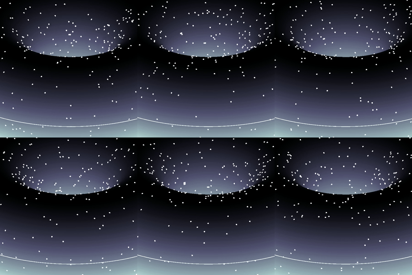
Types of Black Holes:
1. Schwarzschild (Non-rotating, Uncharged):
- This is the simplest type of black hole, described by the Schwarzschild solution.
- Its key feature is the singularity at the center, where the curvature of spacetime becomes infinite.
- No charge, no angular momentum (spin), and spherical symmetry.
2. Kerr (Rotating):
- Describes rotating black holes.
- Involves an additional parameter called angular momentum.
- Has an event horizon and an inner boundary, known as the ergosphere, where spacetime is dragged around by the black hole's rotation.
3. Reissner–Nordström (Charged, Non-rotating):
- A black hole with electric charge.
- A charged black hole has two event horizons (inner and outer) and a central singularity.
4. Kerr–Newman (Rotating and Charged):
- The most general solution, describing a black hole that has both charge and angular momentum.
Relationship Between Schwarzschild Radius and Black Holes
Formation of Black Holes: When a massive star exhausts its nuclear fuel, gravitational collapse can compress the core beyond the Schwarzschild radius, creating a black hole.
Event Horizon: The Schwarzschild radius marks the event horizon for a non-rotating black hole. This is the boundary beyond which no information or matter can escape the black hole.
Curvature of Spacetime: At distances closer than the Schwarzschild radius, spacetime curvature becomes so extreme that all paths, even those of light, are bent towards the black hole’s singularity.
BTW, the term singularity, scientificaly 😊, means that: we do not have a clue what is really happening right there...
Detailed Properties of Black Holes:
a. Singularity:
At the center of a black hole, within the Schwarzschild radius, lies the singularity, a point (or ring in the case of rotating black holes) where gravitational forces compress matter to infinite density and spacetime curvature becomes infinite. General relativity breaks down at the singularity, and a quantum theory of gravity is required for a complete understanding.
b. Event Horizon:
The event horizon is not a physical surface but a boundary where the escape velocity equals the speed of light. For an outside observer, objects falling into a black hole appear to slow down and fade away near the event horizon due to gravitational time dilation, a prediction of general relativity. From the perspective of the infalling object, however, it crosses the event horizon in finite time without noticing anything special at the moment of crossing.
c. Hawking Radiation: (In the post, I told that there is no radiation - to make it simple, although, there is a relatively newly-found (theoretically) radiation. Truth to be said, some physicists are still chalenging this notion, in some of it's parts...)
Quantum mechanical effects near the event horizon predict that black holes can emit radiation (Hawking radiation), a process through which black holes can lose mass and, over very long timescales, potentially evaporate completely. This process has a temperature inversely proportional to the black hole's mass, making large black holes emit extremely weak radiation. (Very trivialy speaking: the concept supposes that an anti-particle is drawn from the vakum and is anihilated with the black's hole matter (particle), and in the process, the black hole looses mass gradually and proportionally to the released energy - very slowly(!)).
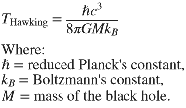
This radiation is significant only for small black holes.
Gravitational Time Dilation (here, as well, things become 'super-weird'...)
Near the Schwarzschild radius, the intense gravitational field leads to time dilation. For an external observer far from the black hole, time appears to slow down for an object moving toward the event horizon. As it approaches the Schwarzschild radius, time dilation becomes so extreme that the object appears frozen in time at the horizon.
The time dilation factor is given by: 

Eg. Approaching the Schwarzschild radius and theoretically remaining just outside of it for a few hours would correspond to the passage of approximately several decades on Earth due to relativistic time dilation.
Using relativistic equations, it's estimated that near the event horizon 2 hours (120 minutes) near the black hole Sagittarius A* (as already mentioned ~ 4 million  ) - in the center of our galaxy Milky Way, could correspond to 83 years passing on Earth! However, this varies based on the precise distance from the event horizon (give or take, a decade 😬).
 ) - in the center of our galaxy Milky Way, could correspond to 83 years passing on Earth! However, this varies based on the precise distance from the event horizon (give or take, a decade 😬).
Information Paradox (definte answer on this question, 'hold's the keys of the universe' 😊, maybe...)
The black hole information paradox arises from the seeming contradiction between general relativity and quantum mechanics.
According to quantum mechanics, information cannot be destroyed, yet anything falling into a black hole seems to be lost beyond the event horizon. Hawking radiation, which allows a black hole to evaporate, does not appear to carry information about the matter that fell into the black hole, leading to ongoing debates and research into how information is preserved in the context of black holes, or not...!
Schwarzschild Radius is the key parameter defining the size of the event horizon of a non-rotating black hole. Black Holes are regions where the Schwarzschild radius constrains all physical phenomena due to extreme gravitational forces, forming event horizons and singularities. The interaction between general relativity and quantum mechanics in the context of black holes (e.g., Hawking radiation and the information paradox) remains one of the most intriguing areas in modern theoretical physics.
For detailed and further reading: https://www.sciencedirect.com/topics/physics-and-astronomy/hawking-radiation.
I hope you will find this post, and information provided, interesting.
This year's MATLAB Shorts Mini Hack contest has kicked off, and there are already lots of interesting entries. The contest features creating a 96-frame, 4-second animation, which is looped 3 times to compose a 12-second short movie. There is an option to add audio to enhance the animation, and it's restricted to a an upper limit of 2,000 characters to promote efficient coding.
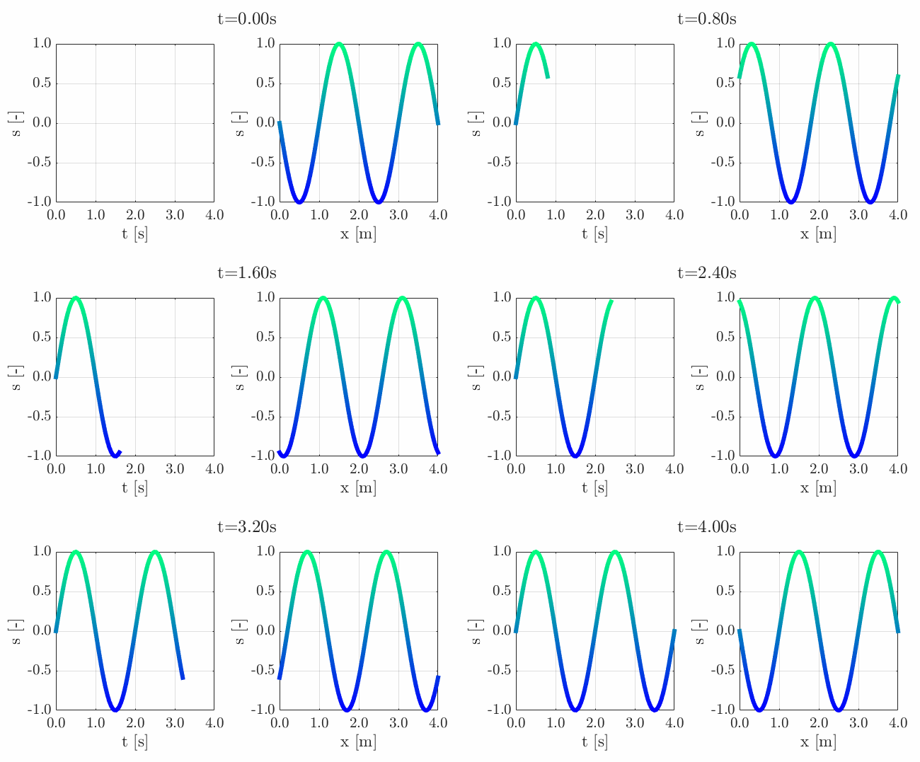
Many of the contestants have already realized the potential for creating a seamless loop, which provides a smooth transition and avoids any discontinuities when the animation is repeated. There are several ways to achieve this. An efficient method for example is utilizing sinusoidal functions, which are periodic, meaning that they repeat themselves over time:
An intuitive example of a seamless loop is @Edgar Guevara's EKG pulse entry, which features an electrocardiogram signal on an oscilloscope. The animation is perfectly matched by the audio, as explained in their post.
Another, rather sophisticated approach is featured in @Tim's Moonrun animation in last year's contest. This seamless loop is achieved by cleverly manipulating the camera position and target over a periodic spatial domain, producing this stunning result:
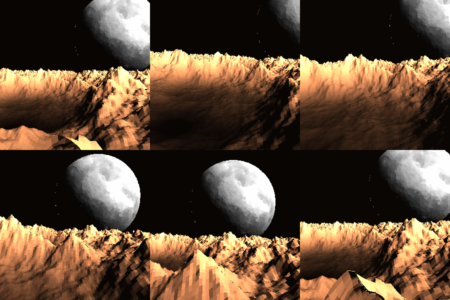
This essentially tells us that for a seamless loop in the spatial domain, the first frame must match the last frame (with a single timestep difference to be more precise, more on that later). But surely this cannot be achieved by zooming in, unless you are simulating a fractal. Well, there are always workarounds.
One way to achieve this is by zooming into a section that contains the first frame of the animation. This is featured in my Winter Loop entry. This is a remix of @Oliver Jaros's Winter entry, which was selected as a one of the weekly winners in the nature & space category for Week 1. The code was modified to lower the character count, but all credits for the original idea and graphics go to them. I also drew inspiration from one of my favourite games of all time, Super Mario 64. Oliver's animation reminded me of the Cool, Cool Mountain level of the game. In the game, you can enter various levels by jumping into paintings serving as portals.
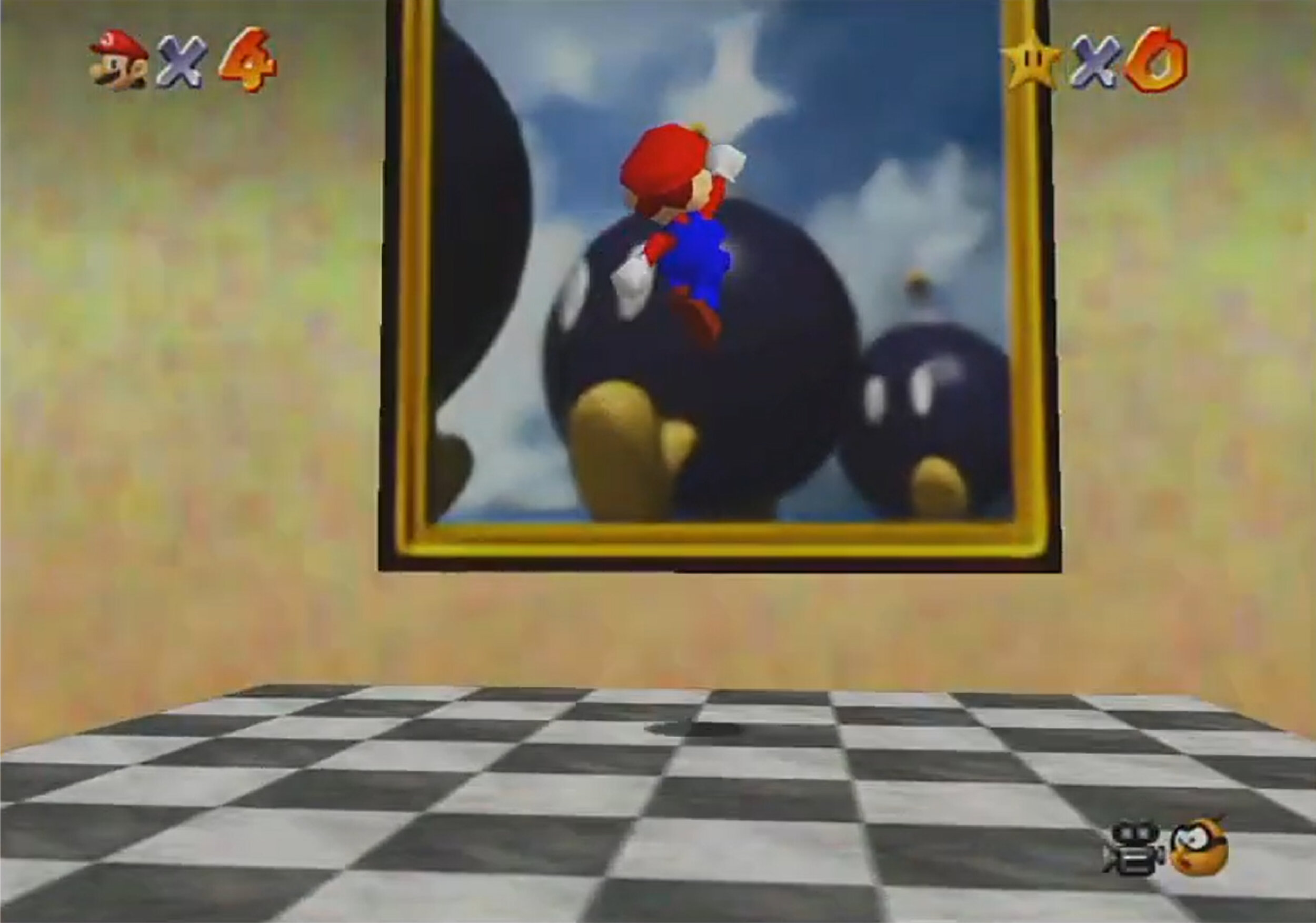
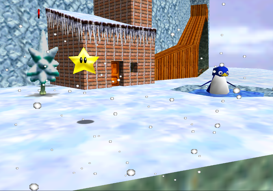
This inspired the idea of zooming into a rectangular photograph frame containing the first frame of the animation to facilitate restarting the loop. One could argue that it would probably take a crazy person to have a photo of their house framed inside their own house. Well, in this economy and with the current house prices, I don't think this scenario is too far-fetched:
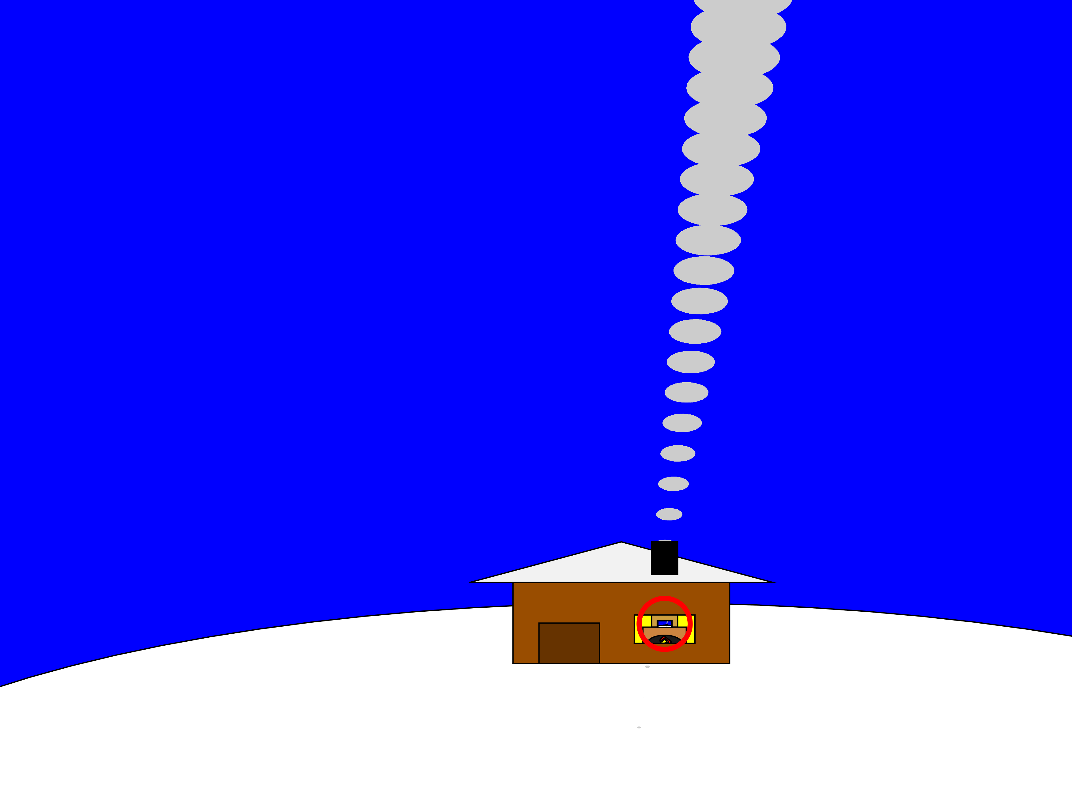
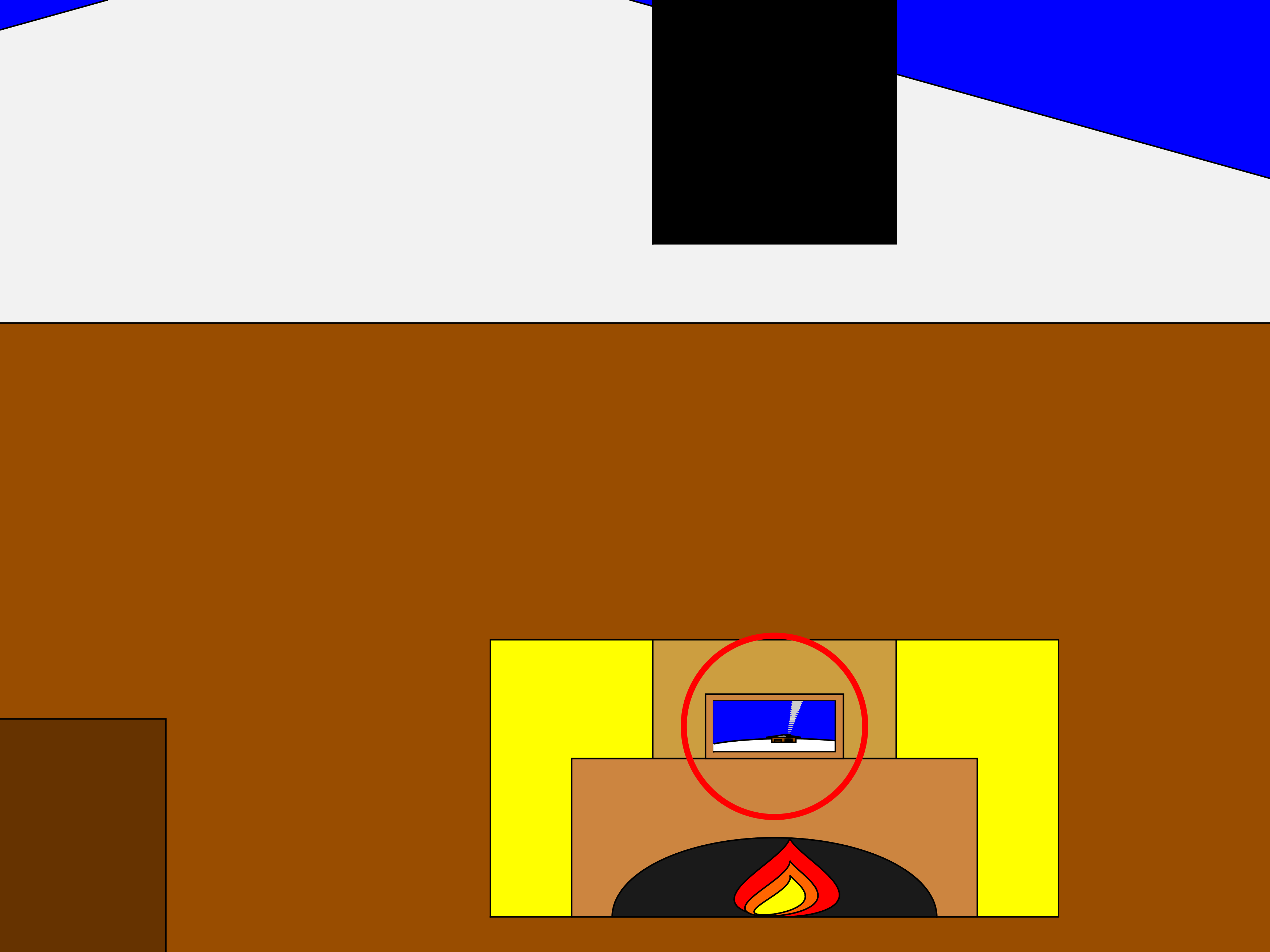
The implementation for this in 2-D is rather simple. Essentially, a second axes is used as the photograph. This is an efficient way of neatly updating the graphics while zooming in. The way this was implemented is explained in the following code snippet, which is a slight modification of the code in the entry:
m = 96; % Number of frames
% Axes limits for the first frame
xm = [xm1,xm2];
ym = [ym1,ym2];
% Axes limits for the last frame (photograph frame edges)
xf = [xf1,xf2];
yf = [yf1,yf2];
% Zoom-in vectors
x1 = linspace(xm(1),xf(1),m+1); % Axes left edge to left photo frame edge
x2 = linspace(xm(2),xf(2),m+1); % Axes right edge to right photo frame edge
y1 = linspace(ym(1),yf(1),m+1); % Axes bottom edge to bottom photo frame edge
y2 = linspace(ym(2),yf(2),m+1); % Axes top edge to top photo frame edge
if f==1
axis([x1(f),x2(f),y1(f),y2(f)]); % Set main axes limits
ax2 = copyobj(gca,gcf); % Create axes for the photo frame containing the first frame graphics objects
end
axis([x1(f+1),x2(f+1),y1(f+1),y2(f+1)]); % Zoom in main axes
lims = axis; % Main axes updated limits
pos = get(gca,'Position'); % Main axes position
% This keeps the relative position of the 2 axes constant:
pos = [pos(1)+diff([lims(1),xf(1)])/diff(lims(1:2))*pos(3),...
pos(2)+diff([lims(3),yf(1)])/diff(lims(3:4))*pos(4),...
diff(xf)/diff(lims(1:2))*pos(3),...
diff(yf)/diff(lims(3:4))*pos(4)];
ax2.Position = pos; % Adjust the relative position
Let's break down the code to explain the process:
- m is the total number of frames in the animation, i.e. 96 frames.
- xm & ym are the main axes limits for frame 1.
- xf & yf are the main axes limits for frame 96, corresponding to the photograph frame's edges.
- x1, x2, y1 & y2 are the zoom-in vectors, linearly spaced from the left, right, bottom & top main axes edges to the corresponding photograph edges. You have probably noticed that these contain m+1=97 points, which is 1 more than the total number of frames. This is done so that the first frame of the animation and the contents of the photograph frame are offset by a single timestep, so that there are no overlapping frames when the animation is looped, thus creating a perfect, seamless loop. That means that the first frame of the animation will contain the main axes zoomed-in by a single timestep, while the last frame of the animation (i.e. the zoomed-in photograph frame) will contain the most zoomed-out version of the graphics. This neatly wraps the animation, and displays the full zoomed-out view when the video stops playing.
- The photograph frame axes are created when f==1 (after setting the initial axes limits) by using the immensely useful copyobj function. This one-liner creates axes containing all graphics objects for the first frame.
- Zooming in on the main axes is then achieved by adjusting the limits using axis([x1(f+1),x2(f+1),y1(f+1),y2(f+1)]). The main axes current limits and position are then saved using the variables lims and pos respectively, in order to adjust the position of the photograph frame axes.
- While zooming in, it's important that the relative position of the 2 axes is kept constant. This is achieved by simply adjusting the position of the photograph frame axes at every frame, by calculating their relative ratios using the abovementioned formula. The first 2 arguments correspond to the (normalized) x and y positions of the lower left corner of the axes, while the third and fourth arguments correspond to the (normalized) width and height respectively. While this formula will work for any position of the main axes, it's a good idea to set the position as set(gca,'Position',[0 0 1 1]) for this contest, in order to take full advantage of the whole allocated window for the animation.
- Finally, note that the graphics are updated for the main axes only, and the above process is repeated for each frame until fully zooming into the photograph frame's axes.
Some of the most curious minds might wonder that while this is well and all with using the second axes to simulate the photograph, what happens to the photograph inside the photograph (and so on...)? Well, the beauty of this method is that you can repeat this as many times as necessary (just apply the formula using the current position and limits of the second axes to adjust the position of the third axes and so on). Given the speed of the animation and the very small size of the photograph inside the photograph, it would be very unlikely that you would need more than 3 axes, but the process is always good to know.
This is the final result:
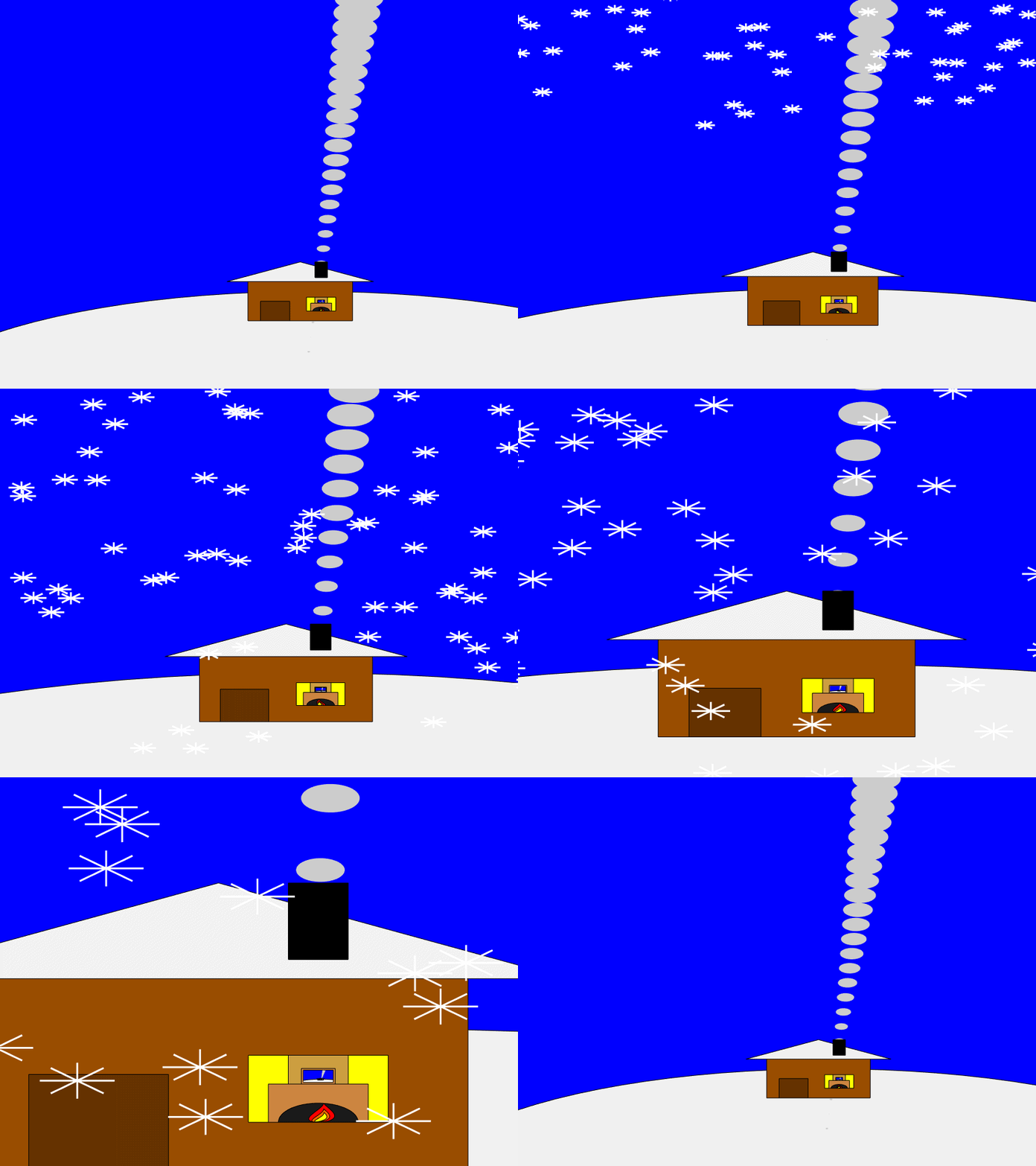
I hope you found these tips useful and I'm looking forward to seeing many creative seamless loop animations in the contest.
Hello! The MathWorks Book Program is thrilled to welcome you to our discussion channel dedicated to books on MATLAB and Simulink. Here, you can:
- Promote Your Books: Are you an author of a book on MATLAB or Simulink? Feel free to share your work with our community. We’re eager to learn about your insights and contributions to the field.
- Request Recommendations: Looking for a book on a specific topic? Whether you're diving into advanced simulations or just starting with MATLAB, our community is here to help you find the perfect read.
- Ask Questions: Curious about the MathWorks Book Program, or need guidance on finding resources? Post your questions and let our knowledgeable community assist you.
We’re excited to see the discussions and exchanges that will unfold here. Whether you're an expert or beginner, there's a place for you in our community. Let's embark on this journey together!
MAThematical LABor
3%
MAth Theory Linear AlgeBra
12.5%
MATrix LABoratory
84%
MATthew LAst Breakthrough
0%
32 votes
At School / university
64%
At work
30%
At home
3%
Elsewhere
3%
33 votes
Here presented MATLAB code is designed to create a seamless loop animation that visualizes an isosurface derived from random data.
This entry, titled "The Scrambled Predator's Cube", builds upon my previous work and has been adapted to include dynamic elements.
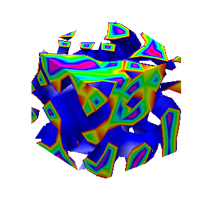
In this explanation, I will break down the relatively short code, making it accessible whether you are a beginner in MATLAB or an experienced user. Let's go through the MATLAB code step by step to understand each line in detail.
Code Breakdown
d = rand(8,8,8);
Random Data Generation: This line creates a three-dimensional array d with dimensions 8×8×8 filled with random values. The rand function generates values uniformly distributed in the interval (0,1). This array serves as the input data for generating the isosurface.
iv = .5 + (f / 10000);
Isovalue Calculation: Here, the isovalue iv is computed based on the frame number f. The expression f / 10000 causes iv to increase very slowly as f increments. Starting from 0.50, this means that for every increment of f, iv changes slightly (specifically, by 0.0001). This gradual increase creates a smooth transition effect in the isosurface over time, making it look dynamic as the animation progresses.
h = patch(isosurface(d, iv), 'FaceColor', 'blue', 'EdgeColor', 'none');
Isosurface Creation: The isosurface function extracts a 3D surface from the data array d at the specified isovalue iv. The result is a patch object h that represents the isosurface in the 3D plot. The 'FaceColor', 'blue' argument sets the face color of the surface to blue, while 'EdgeColor', 'none' specifies that no edges should be drawn, giving the surface a solid appearance.
isonormals(d, h);
Surface Normals Calculation: This function calculates the normals at each vertex of the isosurface h, based on the data in d. Normals are vectors perpendicular to the surface at each point and are crucial for proper lighting calculations. By using isonormals, the appearance of depth and texture is enhanced, allowing the lighting to interact more realistically with the surface.
patch(isocaps(d, iv), 'FaceColor', 'interp', 'EdgeColor', 'none');
Isocaps Visualization: The isocaps function creates flat surfaces (caps) at the boundaries of the isosurface where the data values meet the isovalue iv. The resulting caps are then rendered as patches with 'FaceColor', 'interp', meaning the colors of the caps are interpolated based on the data values. The caps provide a more complete visual representation of the isosurface, improving its overall appearance.
colormap hsv;
Color Map Setup: This line sets the colormap of the current figure to HSV (Hue, Saturation, Value). The HSV colormap allows for a wide range of colors, which can enhance the visual appeal of the rendering by mapping different values in the data to different colors.
daspect([1, 1, 1]);
Aspect Ratio Setting: The daspect function sets the data aspect ratio of the plot to be equal in all three dimensions. This means that one unit in the x-direction is the same length as one unit in the y-direction and z-direction, ensuring that the visual representation of the 3D data is not distorted.
axis tight;
Tight Axis Setting: This command adjusts the limits of the axes so that they fit tightly around the data, removing any excess white space. It helps to focus the viewer's attention on the isosurface and related visual elements.
view(3);
3D View Configuration: The view(3) command sets the current view to a 3D perspective, allowing the viewer to see the structure of the isosurface from an angle that reveals its three-dimensional nature.
camlight right;
camlight left;
Lighting Effects: These commands add two light sources to the scene, positioned to the right and left of the view. The additional lighting enhances the shading and depth perception of the isosurface, making it appear more three-dimensional and visually appealing.
axis off;
Hide Axes: This command turns off the display of the axes in the plot. Removing the axes provides a cleaner visual representation, allowing the viewer to focus solely on the isosurface and its lighting effects without distraction from the grid lines or axis labels.
lighting phong;
Lighting Model: This line sets the lighting model to Phong. The Phong model is widely used in computer graphics as it provides smooth shading and realistic reflections. It calculates how light interacts with surfaces, enhancing the overall appearance by creating a more natural look.
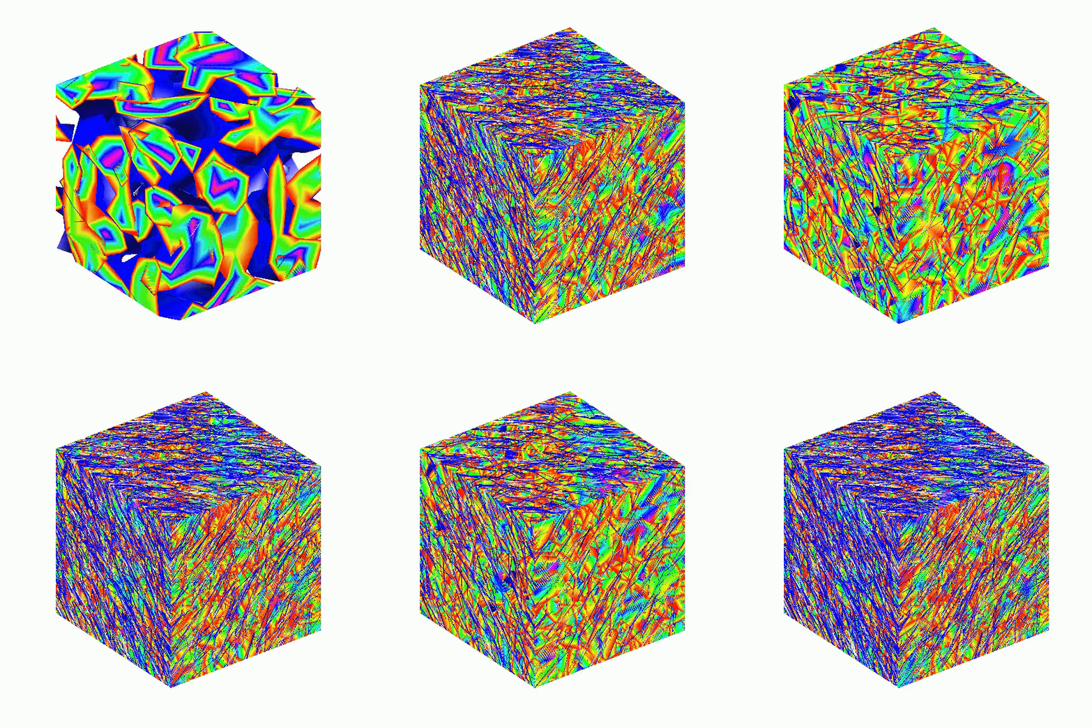
This code creates a visually dynamic and appealing representation of an isosurface derived from random data. The gradual change in the isovalue allows for smooth transitions, while the combination of lighting, colors, and shading contributes to a rich 3D visualization. Each component plays a vital role in rendering the final output, showcasing advanced techniques in data visualization using MATLAB.
I'd like to share some tips about the 2024 mini hack contest, specifically related to audio:
- First (and most important), credit your source: unless you are composing your own audio, I think it's important to give credit to the original sources. It is a little sad to see several contributions with an empty line:
'Cite your audio source here (if applicable):'
- A great place to get royalty-free and high-quality music and audio (among other media) is https://pixabay.com. Be sure to check it out! I used one of their audio clips in my submission EKG pulse
- The right music can enhance the overall experience of your animation. Sometimes getting the animation to match the music beat can be hard. I suggest you try the other way around: get your music/sound effects to match the animation rhythm with a little editing. A free audio editor with many capabilities (more than enough for this contest, I think) is https://www.audacityteam.org/
- Choose a 4-second audio clip with a consistent tempo and seamless loop points, ensuring it complements your animation's mood and loops smoothly over 12 seconds without abrupt changes.
I think that when the right music is paired with the right animation, it can create a more impactful experience.
Well, this is my first time to participate in such community competitions and guess what, I've gone for 4 submissions so far (Feels Great!!)
So I wanna share some tricks that I followed for my first submission named Happy Shaping' ( Go Check it out!!):
1. Dynamic Background Color Change:
- Technique: The background color of the figure window is gradually changed using sine and cosine functions.
- Reason: These trigonometric functions (sin and cos) create smooth, oscillating transitions over time, which gives a fluid effect to the background's color shift.
- Implementation:
Color = [0.1 + 0.5*abs(sin(f/10)), 0.1 + 0.5*abs(cos(f/15)), 0.9 -
0.5*abs(sin(f/20))];
- Benefit: This introduces a smooth, visually appealing animation effect.
2. Smooth Object Motion Using Sine and Cosine:
- Technique: The position and shape of objects are based on trigonometric functions.
- Reason: Using sin(t) and cos(t) ensures that the movement is circular or elliptical, creating continuous and natural motion in animations.
- Implementation (for object position):
x = 10 * cos(t * 2 * pi) * (1 + 0.5 * sin(t * pi));
y = 10 * sin(t * 2 * pi) * (1 + 0.5 * cos(t * pi));
- Benefit: Circular and smooth motions are pleasing and easily controlled by tweaking the frequency and phase of sine/cosine functions.
3. Polygon Shape Changing Over Time:
- Technique: The number of sides of the polygon (sides) changes dynamically based on t.
- Reason: It creates variation in shape, maintaining user interest as the shape transitions from a triangle to a hexagon.
- Implementation:
sides = 3 + round(3 * abs(sin(t)));
- Benefit: This provides dynamic shape transitions over time, keeping the animation non-static.
4. Use of the fill Function for Color-Filled Shapes:
- Technique: The fill function is used to draw a polygon with smoothly changing colors.
- Reason: Filling polygons with varying colors based on time (t) allows for continuous color transitions, adding more complexity to the animation.
- Implementation:
fill(xp, yp, c, 'EdgeColor', 'none');
- Benefit: Combining both color changes and shape changes enhances the visual impact.
5. Consistent Use of hold on and hold off:
- Technique: hold on allows multiple graphic objects to be drawn on the same axes without clearing previous objects.
- Reason: This is crucial for drawing multiple elements (like polygons, circles, and lines) on the same figure.
- Benefit: It helps manage and layer different graphical elements effectively within the same frame.
6. Use of rectangle for a Smooth Ball Motion:
- Technique: The ball's motion is defined by rectangle with a Curvature of [1, 1] to make it circular.
- Reason: Using the rectangle function simplifies the process of drawing a filled circle, and controlling its position and size is intuitive.
- Benefit: It provides a straightforward way to animate circular objects within the plot.
7. Animating the Connection Line:
- Technique: A white dashed line (w--) is drawn between the polygon and the moving ball to show a connection between these objects.
- Reason: This adds interactivity to the scene, as it gives the impression that the polygon and the ball are related or connected in some way.
- Implementation:
plot([x bx], [y by], 'w--', 'LineWidth', 2);
- Benefit: A dynamic element that adds depth and narrative to the animation, guiding the viewer’s attention.
8. Frame Synchronization with Time (f and t):
- Technique: The variable f is used as a frame number, while t = f / 24 creates a link between frame and time.
- Reason: Ensuring smooth and continuous transitions in the animation over time is critical, so f acts as the control for time-based changes in shape, color, and position.
- Benefit: This makes it easy to manage frame rates and time-based updates for the animation.
If you like them, please feel free to use them for free.
function drawframe(f)
% Create a figure
figure;
hold on;
axis equal;
axis off;
% Draw the roads
rectangle('Position', [0, 0, 2, 30], 'FaceColor', [0.5 0.5 0.5]); % Left road
rectangle('Position', [2, 0, 2, 30], 'FaceColor', [0.5 0.5 0.5]); % Right road
% Draw the traffic light
trafficLightPole = rectangle('Position', [-1, 20, 1, 0.2], 'FaceColor', 'black'); % Pole
redLight = rectangle('Position', [0, 20, 0.5, 1], 'FaceColor', 'red'); % Red light
yellowLight = rectangle('Position', [0.5, 20, 0.5, 1], 'FaceColor', 'black'); % Yellow light
greenLight = rectangle('Position', [1, 20, 0.5, 1], 'FaceColor', 'black'); % Green light
carBody = rectangle('Position', [2.5, 2, 1, 4], 'Curvature', 0.2, 'FaceColor', 'red'); % Body
leftWheel = rectangle('Position', [2.5, 3.0, 0.2, 0.2], 'Curvature', [1, 1], 'FaceColor', 'black'); % Left wheel
rightWheel = rectangle('Position', [3.3, 3.0, 0.2, 0.2], 'Curvature', [1, 1], 'FaceColor', 'black'); % Right wheel
leftFrontWheel = rectangle('Position', [2.5, 5.0, 0.2, 0.2], 'Curvature', [1, 1], 'FaceColor', 'black'); % Left wheel
rightFrontWheel = rectangle('Position', [3.3, 5.0, 0.2, 0.2], 'Curvature', [1, 1], 'FaceColor', 'black'); % Right wheel
% Set limits
xlim([-1, 8]);
ylim([-1, 35]);
% Animation parameters
carSpeed = 0.5; % Speed of the car
carPosition = 2; % Initial car position
stopPosition = 15; % Position to stop at the traffic light
isStopped = false; % Car is not stopped initially
%Animation loop
for t = 1:100
% Update traffic light: Red for 40 frames, yellow for 10 frames Green for 40 frames
if t <= 40
% Red light on, yellow and green off
set(redLight, 'FaceColor', 'red');
set(yellowLight, 'FaceColor', 'black');
set(greenLight, 'FaceColor', 'black');
elseif t > 40 && t <= 50
% Change to green light
set(redLight, 'FaceColor', 'black');
set(yellowLight, 'FaceColor', 'yellow');
set(greenLight, 'FaceColor', 'black');
else
% Back to red light
set(redLight, 'FaceColor', 'black');
set(yellowLight, 'FaceColor', 'black');
set(greenLight, 'FaceColor', 'green');
isStopped = false; % Allow car to move
end
%Move the car
if ~isStopped
carPosition = carPosition + carSpeed; % Move forward
if carPosition < stopPosition
%do nothing
else
isStopped = true;
end
else
% Gradually stop the car when red
if carPosition > stopPosition
carPosition = carPosition + carSpeed*(1-t/50); % Move backward until it reaches the stop position
end
end
if carPosition >= 25
carPosition = 25;
end
% Update car position
% set(carBody, 'Position', [carPosition, 2, 1, 0.5]);
set(carBody, 'Position', [2.5, carPosition, 1, 4]);
%set(carWindow, 'Position', [carPosition + 0.2, 2.4, 0.6, 0.2]);
%set(leftWheel, 'Position', [carPosition, 1.5, 0.2, 0.2]);
set(leftWheel, 'Position', [2.5, carPosition+1, 0.2, 0.2]);
% set(rightWheel, 'Position', [carPosition + 0.8, 1.5, 0.2, 0.2]);
set(rightWheel, 'Position', [3.3, carPosition+1, 0.2, 0.2]);
set(leftFrontWheel, 'Position', [2.5, carPosition+3, 0.2, 0.2]);
set(rightFrontWheel, 'Position', [3.3, carPosition+3, 0.2, 0.2]);
% Pause to control animation speed
pause(0.01);
end
hold off;
Let's say you have a chance to ask the MATLAB leadership team any question. What would you ask them?
What is the side-effect of counting the number of Deep Learning Toolbox™ updates in the last 5 years? The industry has slowly stabilised and matured, so updates have slowed down in the last 1 year, and there has been no exponential growth.Is it correct to assume that? Let's see what you think!
releaseNumNames = "R"+string(2019:2024)+["a";"b"];
releaseNumNames = releaseNumNames(:);
numReleaseNotes = [10,14,27,39,38,43,53,52,55,57,46,46];
exampleNums = [nan,nan,nan,nan,nan,nan,40,24,22,31,24,38];
bar(releaseNumNames,[numReleaseNotes;exampleNums]')
legend(["#release notes","#new/update examples"],Location="northwest")
title("Number of Deep Learning Toolbox™ update items in the last 5 years")
ylabel("#release notes")

See the attached PDF for a higher resolution
Related blogs posts:
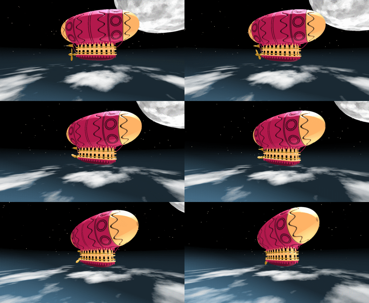
In the spirit of warming up for this year's minihack contest, I'm uploading a walkthrough for how to design an airship using pure Matlab script. This is commented and uncondensed; half of the challenge for the minihacks is how minimize characters. But, maybe it will give people some ideas.
The actual airship design is from one of my favorite original NES games that I played when I was a kid - Little Nemo: The Dream Master. The design comes from the intro of the game when Nemo sees the Slumberland airship leave for Slumberland:
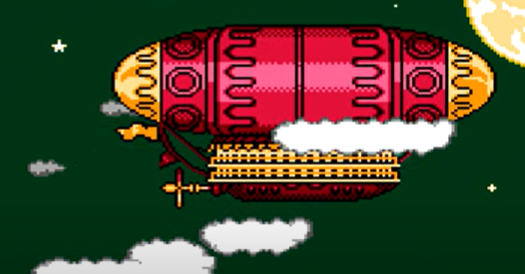
(Snip from a frame of the opening scene in Capcom's game Little Nemo: The Dream Master, showing the Slumberland airship).
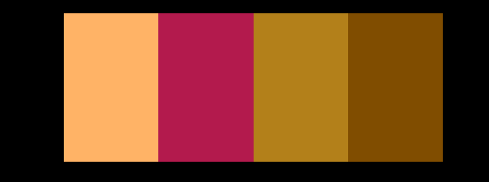
I spent hours playing this game with my two sisters, when we were little. It's fun and tough, but the graphics sparked the imagination. On to the code walkthrough, beginning with the color palette: these four colors are the only colors used for the airship:
c1=cat(3,1,.7,.4); % Cream color
c2=cat(3,.7,.1,.3); % Magenta
c3=cat(3,0.7,.5,.1); % Gold
c4=cat(3,.5,.3,0); % bronze
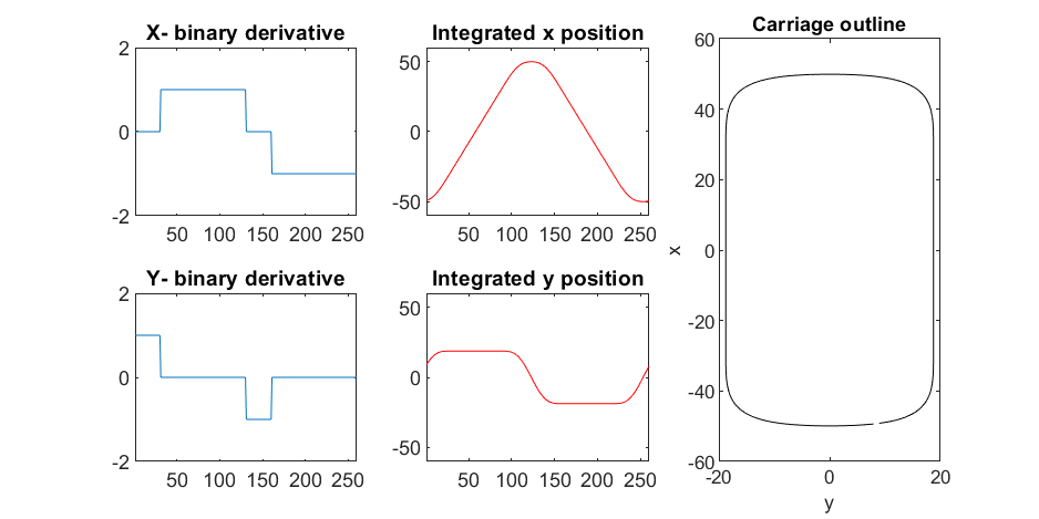
We start with the airship carriage body. We want something rectangular but smoothed on the corners. To do this we are going to start with the separate derivatives of the x and y components, which can be expressed using separate blocks of only three levels: [1, 0, -1]. You could integrate to create a rectangle, but if we smooth the derivatives prior to integrating we will get rounded edges. This is done in the following code:
% Binary components for x & y vectors
z=zeros(1,30);
o=ones(1,100);
% X and y vectors
x=[z,o,z,-o];
y=[1+z,1-o,z-1,1-o];
% Smoother function (fourier / circular)
s=@(x)ifft(fft(x).*conj(fft(hann(45)'/22,260)));
% Integrator function with replication and smoothing to form mesh matrices
u=@(x)repmat(cumsum(s(x)),[30,1]);
% Construct x and y components of carriage with offsets
x3=u(x)-49.35;
y3=u(y)+6.35;
y3 = y3*1.25; % Make it a little fatter
% Add a z-component to make the full set of matrices for creating a 3D
% surface:
z3=linspace(0,1,30)'.*ones(1,260)*30;
z3(14,:)=z3(15,:); % These two lines are for adding platforms
z3(2,:)=z3(3,:); % to the carriage, later.
Plotting x, y, and the top row of the smoothed, integrated, and replicated matrices x3 and y3 gives the following:
We now have the x and y components for a 3D mesh of the carriage, let's make it more interesting by adding a color scheme including doors, and texture for the trim around the doors. Let's also add platforms beneath the doors for passengers to walk on.
Starting with the color values, let's make doors by convolving points in a color-matrix by a door shaped function.
m=0*z3; % Image matrix that will be overlayed on carriage surface
m(7,10:12:end)=1; % Door locations (lower deck)
m(21,10:12:end)=1; % Door locations (upper deck)
drs = ones(9, 5); % Door shape
m=1-conv2(m,ones(9,5),'same'); % Applying
To add the trim, we will convolve matrix "m" (the color matrix) with a square function, and look for values that lie between the extrema. We will use this to create a displacement function that bumps out the -x, and -y values of the carriage surface in intermediary polar coordinate format.
rm=conv2(m,ones(5)/25,'same'); % Smoothing the door function
rm(~m)=0; % Preserving only the region around the doors
rds=0*m; % Radial displacement function
rds(rm<1&rm>0)=1; % Preserving region around doors
rds(m==0)=0;
rds(13:14,:)=6; % Adding walkways
rds(1:2,:)=6;
% Apply radial displacement function
[th,rd]=cart2pol(x3,y3);
[x3T,y3T]=pol2cart(th,(rd+rds)*.89);
If we plot the color function (m) and radial displacement function (rds) we get the following:
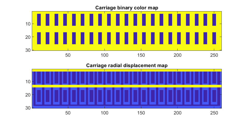
In the upper plot you can see the doors, and in the bottom map you can see the walk way and door trim.
Next, we are going to add some flags draped from the bottom and top of the carriage. We are going to recycle the values in "z3" to do this, by multiplying that matrix with the absolute value of a sine-wave, squished a bit with the soft-clip erf() function.
We add a keel to the airship carriage using a canonical sphere turned on its side, again using the soft-clip erf() function to make it roughly rectangular in x and y, and multiplying with a vector that is half nan's to make the top half transparent.
At this point, since we are beginning the plotting of the ship, we also need to create our hgtransform objects. These allow us to move all of the components of the airship in unison, and also link objects with pivot points to the airship, such as the propeller.
% Now we need some flags extending around the top and bottom of the
% carriage. We can do this my multiplying the height function (z3) with the
% absolute value of a sine-wave, rounded with a compression function
% (erf() in this case);
g=-z3.*erf(abs(sin(linspace(0,40*pi,260))))/4; % Flags
% Also going to add a slight taper to the carriage... gives it a nice look
tp=linspace(1.05,1,30)';
% Finally, plotting. Plot the carriage with the color-map for the doors in
% the cream color, than the flags in magenta. Attach them both to transform
% objects for movement.
% Set up transform objects. 2 moving parts:
% 1) The airship itself and all sub-components
% 2) The propellor, which attaches to the airship and spins on its axis.
hold on;
P=hgtransform('Parent',gca); % Ship
S=hgtransform('Parent',P); % Prop
surf(x3T.*tp,y3T,z3,c1.*m,'Parent',P);
surf(x3,y3,g,c2.*rd./rd, 'Parent', P);
surf(x3,y3,g+31,c2.*rd./rd, 'Parent', P);
axis equal
% Now add the keel of the airship. Will use a canonical sphere and the
% erf() compression function to square off.
[x,y,z]=sphere(99);
mk=round(linspace(-1,1).^2+.3); % This function makes the top half of the sphere nan's for transparency.
surf(50*erf(1.4*z),15*erf(1.4*y),13*x.*mk./mk-1,.5*c2.*z./z, 'Parent', P);
% The carriage is done. Now we can make the blimp above it.
We haven't adjusted the shading of the image yet, but you can see the design features that have been created:
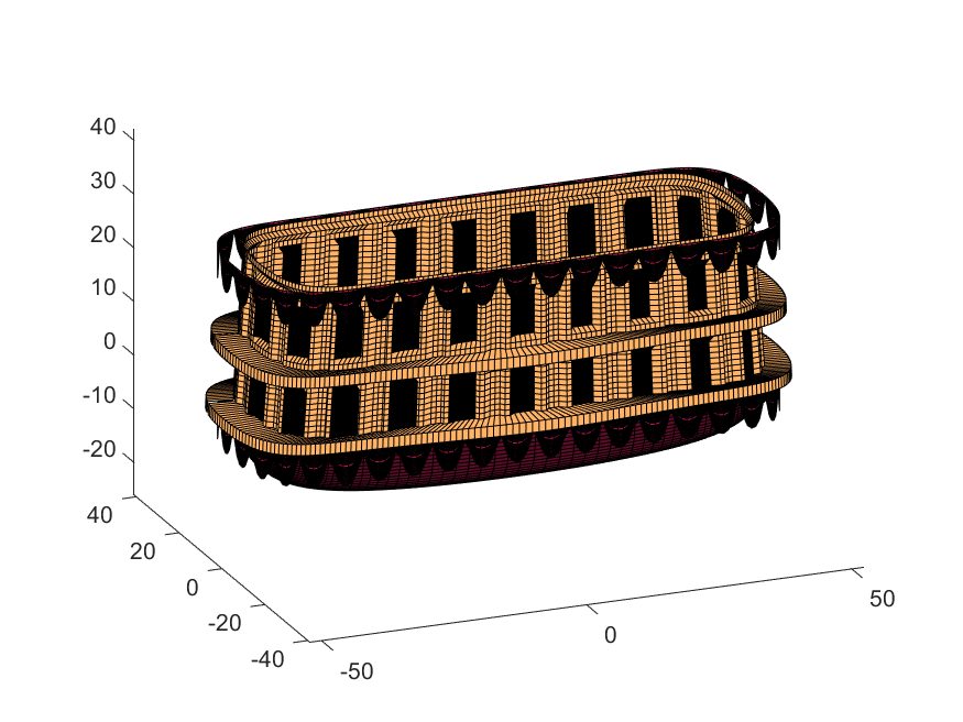
Next, we start working on the blimp. This is going to use a few more vertices & faces. We are going to use a tapered cylinder for this part, and will start by making the overlaid image, which will have 2 colors plus radial rings, circles, and squiggles for ornamentation.
M=525; % Blimp (matrix dimensions)
N=700;
% Assign the blimp the cream and magenta colors
t=122; % Transition point
b=ones(M,N,3); % Blimp color map template
bc=b.*c1; % Blimp color map
bc(:,t+1:end-t,:)=b(:,t+1:end-t,:).*c2;
% Add axial rings around blimp
l=[.17,.3,.31,.49];
l=round([l,1-fliplr(l)]*N); % Mirroring
lnw=ones(1,N); % Mask
lnw(l)=0;
lnw=rescale(conv(lnw,hann(7)','same'));
bc=bc.*lnw;
% Now add squiggles. We're going to do this by making an even function in
% the x-dimension (N, 725) added with a sinusoidal oscillation in the
% y-dimension (M, 500), then thresholding.
r=sin(linspace(0, 2*pi, M)*10)'+(linspace(-1, 1, N).^6-.18)*15;
q=abs(r)>.15;
r=sin(linspace(0, 2*pi, M)*12)'+(abs(linspace(-1, 1, N))-.25)*15;
q=q.*(abs(r)>.15);
% Now add the circles on the blimp. These will be spaced evenly in the
% polar angle dimension around the axis. We will have 9. To make the
% circles, we will create a cone function with a peak at the center of the
% circle, and use thresholding to create a ring of appropriate radius.
hs=[1,.75,.5,.25,0,-.25,-.5,-.75,-1]; % Axial spacing of rings
% Cone generation and ring loop
xy= @(h,s)meshgrid(linspace(-1, 1, N)+s*.53,(linspace(-1, 1, M)+h)*1.15);
w=@(x,y)sqrt(x.^2+y.^2);
for n=1:9
h=hs(n);
[xx,yy]=xy(h,-1);
r1=w(xx,yy);
[xx,yy]=xy(h,1);
r2=w(xx,yy);
b=@(x,y)abs(y-x)>.005;
q=q.*b(.1,r1).*b(.075,r1).*b(.1,r2).*b(.075,r2);
end
The figures below show the color scheme and mask used to apply the squiggles and circles generated in the code above:
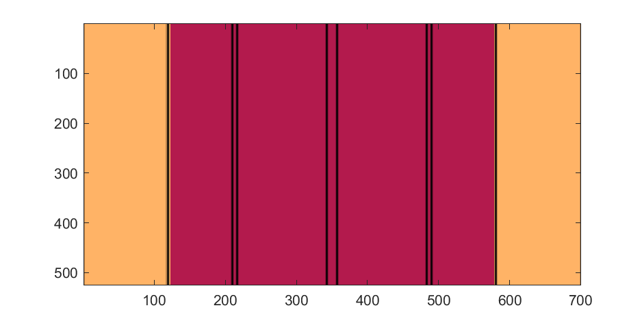
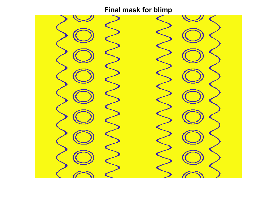
Finally, for the colormap we are going to smooth the binary mask to avoid hard transitions, and use it to to add a "puffy" texture to the blimp shape. This will be done by diffusing the mask iteratively in a loop with a non-linear min() operator.
% 2D convolution function
ff=@(x)circshift(ifft2(fft2(x).*conj(fft2(hann(7)*hann(7)'/9,M,N))),[3,3]);
q=ff(q); % Smooth our mask function
hh=rgb2hsv(q.*bc); % Convert to hsv: we are going to use the value
% component for radial displacement offsets of the
% 3D blimp structure.
rd=hh(:,:,3); % Value component
for n=1:10
rd=min(rd,ff(rd)); % Diffusing the value component for a puffy look
end
rd=(rd+35)/36; % Make displacements effects small
% Now make 3D blimp manifold using "cylinder" canonical shape
[x,y,z]=cylinder(erf(sin(linspace(0,pi,N)).^.5)/4,M-1); % First argument is the blimp taper
[t,r]=cart2pol(x, y);
[x2,y2]=pol2cart(t, r.*rd'); % Applying radial displacment from mask
s=200;
% Plotting the blimp
surf(z'*s-s/2, y2'*s, x2'*s+s/3.9+15, q.*bc,'Parent',P);
Notice that the parent of the blimp surface plot is the same as the carriage (e.g. hgtransform object "P"). Plotting at this point using flat shading and adding some lighting gives the image below:
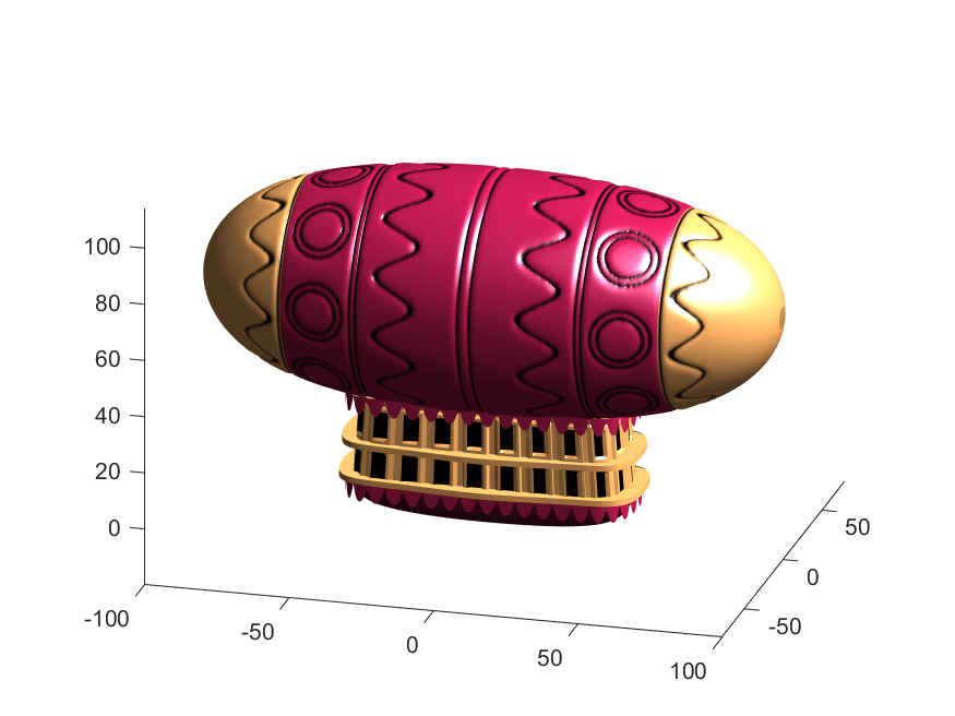
Next, we need to add a propeller so it can move. This will include the creation of a shaft using the cylinder() function. The rest of the pieces (the propeller blades, collars and shaft tip) all use the same canonical sphere with distortions applied using various math functions. Note that when the propeller is made it is linked to hgtransform object "S" rather than "P." This will allow the propeller to rotate, but still be joined to the airship.
% Next, the propeller. First, we start with the shaft. This is a simple
% cylinder. We add an offset variable and a scale variable to move our
% propeller components around, as well.
shx = -70; % This is our x-shifter for components
scl = 3; % Component size scaler
[x,y,z]=cylinder(1, 20); % Canonical cylinder for prop shaft.
p(1)=surf(-scl*(z-1)*7+shx,scl*x/2,scl*y/2,0*x+c4,'Parent',P); % Prop shaft
% Now the propeller. This is going to be made from a distorted sphere.
% The important thing here is that it is linked to the "S" hgtransform
% object, which will allow it to rotate.
[x,y,z]=sphere(50);
a=(-1:.04:1)';
x2=(x.*cos(a)-y/3.*sin(a)).*(abs(sin(a*2))*2+.1);
y2=(x.*sin(a)+y/3.*cos(a));
p(2)=surf(-scl*y2+shx,scl*x2,scl*z*6,0*x+c3,'Parent',S);
% Now for the prop-collars. You can see these on the shaft in the NES
% animation. These will just be made by using the canonical sphere and the
% erf() activation function to square it in the x-dimension.
g=erf(z*3)/3;
r=@(g)surf(-scl*g+shx,scl*x,scl*y,0*x+c3,'Parent',P);
r(g);
r(g-2.8);
r(g-3.7);
% Finally, the prop shaft tip. This will just be the sphere with a
% taper-function applied radially.
t=1.7*cos(0:.026:1.3)'.^2;
p(3)=surf(-(z*2+2)*scl + shx,x.*t*scl,y.*t*scl, 0*x+c4,'Parent',P);
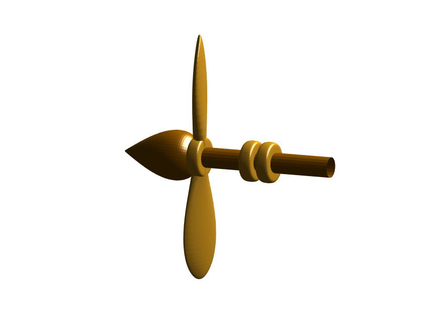
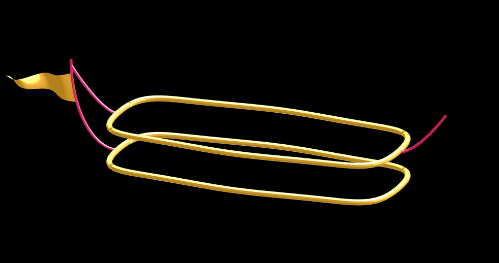
Now for some final details including the ropes to the blimp, a flag hung on one of the ropes, and railings around the walkways so that passengers don't plummet to their doom. This will make use of the ad-hoc "ropeG" function, which takes a 3D vector of points and makes a conforming cylinder around it, so that you get lighting functions etc. that don't work on simple lines. This function is added to the script at the end to do this:
% Rope function for making a 3D curve have thickness, like a rope.
% Inputs:
% - xyz (3D curve vector, M points in 3 x M format)
% - N (Number of radial points in cylinder function around the curve
% - W (Width of the rope)
%
% Outputs:
% - xf, yf, zf (Matrices that can be used with surf())
function [xf, yf, zf] = RopeG(xyz, N, W)
% Canonical cylinder with N points in circumference
[xt,yt,zt] = cylinder(1, N);
% Extract just the first ring and make (W) wide
xyzt = [xt(1, :); yt(1, :); zt(1, :)]*W;
% Get local orientation vector between adjacent points in rope
dxyz = xyz(:, 2:end) - xyz(:, 1:end-1);
dxyz(:, end+1) = dxyz(:, end);
vcs = dxyz./vecnorm(dxyz);
% We need to orient circle so that its plane normal is parallel to
% xyzt. This is a kludgey way to do that.
vcs2 = [ones(2, size(vcs, 2)); -(vcs(1, :) + vcs(2, :))./(vcs(3, :)+0.01)];
vcs2 = vcs2./vecnorm(vcs2);
vcs3 = cross(vcs, vcs2);
p = @(x)permute(x, [1, 3, 2]);
rmats = [p(vcs3), p(vcs2), p(vcs)];
% Create surface
xyzF = pagemtimes(rmats, xyzt) + permute(xyz, [1, 3, 2]);
% Outputs for surf format
xf = squeeze(xyzF(1, :, :));
yf = squeeze(xyzF(2, :, :));
zf = squeeze(xyzF(3, :, :));
end
Using this function we can define the ropes and balconies. Note that the balconies simply recycle one of the rows of the original carriage surface, defining the outer rim of the walkway, but bumping up in the z-dimension.
cb=-sqrt(1-linspace(1, 0, 100).^2)';
c1v=[linspace(-67, -51)', 0*ones(100,1),cb*30+35];
c2v=[c1v(:,1),c1v(:,2),(linspace(1,0).^1.5-1)'*15+33];
c3v=c2v.*[-1,1,1];
[xr,yr,zr]=RopeG(c1v', 10, .5);
surf(xr,yr,zr,0*xr+c2,'Parent',P);
[xr,yr,zr]=RopeG(c2v', 10, .5);
surf(xr,yr,zr,0*zr+c2,'Parent',P);
[xr,yr,zr]=RopeG(c3v', 10, .5);
surf(xr,yr,zr,0*zr+c2,'Parent',P);
% Finally, balconies would add a nice touch to the carriage keep people
% from falling to their death at 10,000 feet.
[rx,ry,rz]=RopeG([x3T(14, :); y3T(14,:); 0*x3T(14,:)+18]*1.01, 10, 1);
surf(rx,ry,rz,0*rz+cat(3,0.7,.5,.1),'Parent',P);
surf(rx,ry,rz-13,0*rz+cat(3,0.7,.5,.1),'Parent',P);
And, very last, we are going to add a flag attached to the outer cable. Let's make it flap in the wind. To make it we will recycle the z3 matrix again, but taper it based on its x-value. Then we will sinusoidally oscillate the flag in the y dimension as a function of x, constraining the y-position to be zero where it meets the cable. Lastly, we will displace it quadratically in the x-dimension as a function of z so that it lines up nicely with the rope. The phase of the sine-function is modified in the animation loop to give it a flapping motion.
h=linspace(0,1);
sc=10;
[fx,fz]=meshgrid(h,h-.5);
F=surf(sc*2.5*fx-90-2*(fz+.5).^2,sc*.3*erf(3*(1-h)).*sin(10*fx+n/5),sc*fz.*h+25,0*fx+c3,'Parent',P);
Plotting just the cables and flag shows:
Putting all the pieces together reveals the full airship:
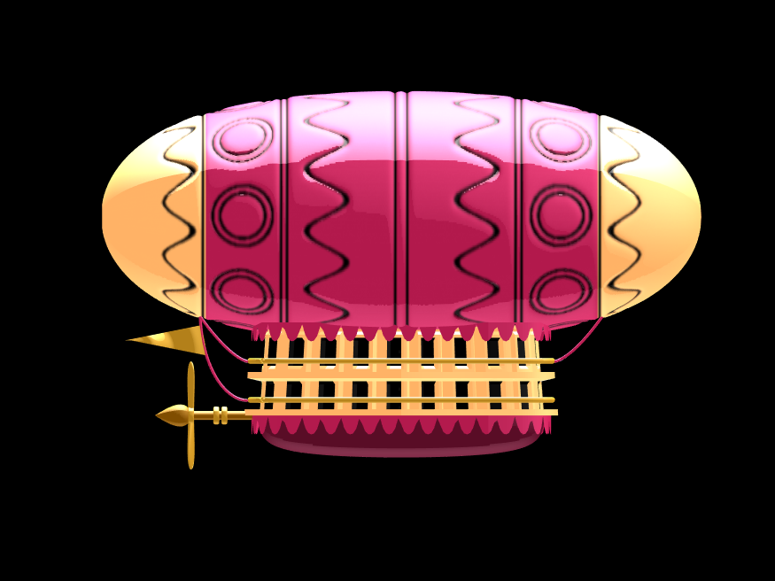
A note about lighting: lighting and material properties really change the feel of the image you create. The above picture is rendered in a cartoony style by setting the specular exponent to a very low value (1), and adding lots of diffuse and ambient reflectivity as well. A light below the airship was also added, albeit with lower strength. Settings used for this plot were:
shading flat
view([0, 0]);
L=light;
L.Color = [1,1,1]/4;
light('position', [0, 0.5, 1], 'color', [1,1,1]);
light('position', [0, 1, -1], 'color', [1, 1, 1]/5);
material([1, 1, .7, 1])
set(gcf, 'color', 'k');
axis equal off
What about all the rest of the stuff (clouds, moon, atmospheric haze etc.) These were all (mostly) recycled bits from previous minihack entries. The clouds were made using power-law noise as explained in Adam Danz' blog post. The moon was borrowed from moonrun, but with an increased number of points. Atmospheric haze was recycled from Matlon5. The rest is just camera angles, hgtransform matrix updates, and updating alpha-maps or vertex coordinates.
Finally, the use of hann() adds the signal processing toolbox as a dependency. To avoid this use the following anonymous function:
hann = @(x)-cospi(linspace(0,2,x)')/2+.5;
Create a struct arrays where each struct has field names "a," "b," and "c," which store different types of data. What efficient methods do you have to assign values from individual variables "a," "b," and "c" to each struct element? Here are five methods I've provided, listed in order of decreasing efficiency. What do you think?
Create an array of 10,000 structures, each containing each of the elements corresponding to the a,b,c variables.
num = 10000;
a = (1:num)';
b = string(a);
c = rand(3,3,num);
Here are the methods;
%% method1
t1 =tic;
s = struct("a",[], ...
"b",[], ...
"c",[]);
s1 = repmat(s,num,1);
for i = 1:num
s1(i).a = a(i);
s1(i).b = b(i);
s1(i).c = c(:,:,i);
end
t1 = toc(t1);
%% method2
t2 =tic;
for i = num:-1:1
s2(i).a = a(i);
s2(i).b = b(i);
s2(i).c = c(:,:,i);
end
t2 = toc(t2);
%% method3
t3 =tic;
for i = 1:num
s3(i).a = a(i);
s3(i).b = b(i);
s3(i).c = c(:,:,i);
end
t3 = toc(t3);
%% method4
t4 =tic;
ct = permute(c,[3,2,1]);
t = table(a,b,ct);
s4 = table2struct(t);
t4 = toc(t4);
%% method5
t5 =tic;
s5 = struct("a",num2cell(a),...
"b",num2cell(b),...
"c",squeeze(mat2cell(c,3,3,ones(num,1))));
t5 = toc(t5);
%% plot
bar([t1,t2,t3,t4,t5])
xtickformat('method %g')
ylabel("time(second)")
yline(mean([t1,t2,t3,t4,t5]))
Hot off the heels of my High Performance Computing experience in the Czech republic, I've just booked my flights to Atlanta for this year's supercomputing conference at SC24.
Will any of you be there?
syms u v
atan2alt(v,u)
function Z = atan2alt(V,U)
% extension of atan2(V,U) into the complex plane
Z = -1i*log((U+1i*V)./sqrt(U.^2+V.^2));
% check for purely real input. if so, zero out the imaginary part.
realInputs = (imag(U) == 0) & (imag(V) == 0);
Z(realInputs) = real(Z(realInputs));
end
As I am editing this post, I see the expected symbolic display in the nice form as have grown to love. However, when I save the post, it does not display. (In fact, it shows up here in the discussions post.) This seems to be a new problem, as I have not seen that failure mode in the past.
You can see the problem in this Answer forum response of mine, where it did fail.
In case you haven't come across it yet, @Gareth created a Jokes toolbox to get MATLAB to tell you a joke.
I was browsing the MathWorks website and decided to check the Cody leaderboard. To my surprise, William has now solved 5,000 problems. At the moment, there are 5,227 problems on Cody, so William has solved over 95%. The next competitor is over 500 problems behind. His score is also clearly the highest, approaching 60,000.


