Results for
I got thoroughly nerd-sniped by this xkcd, leading me to wonder if you can use MATLAB to figure out the dice roll for any given (rational) probability. Well, obviously you can. The question is how. Answer: lots of permutation calculations and convolutions.
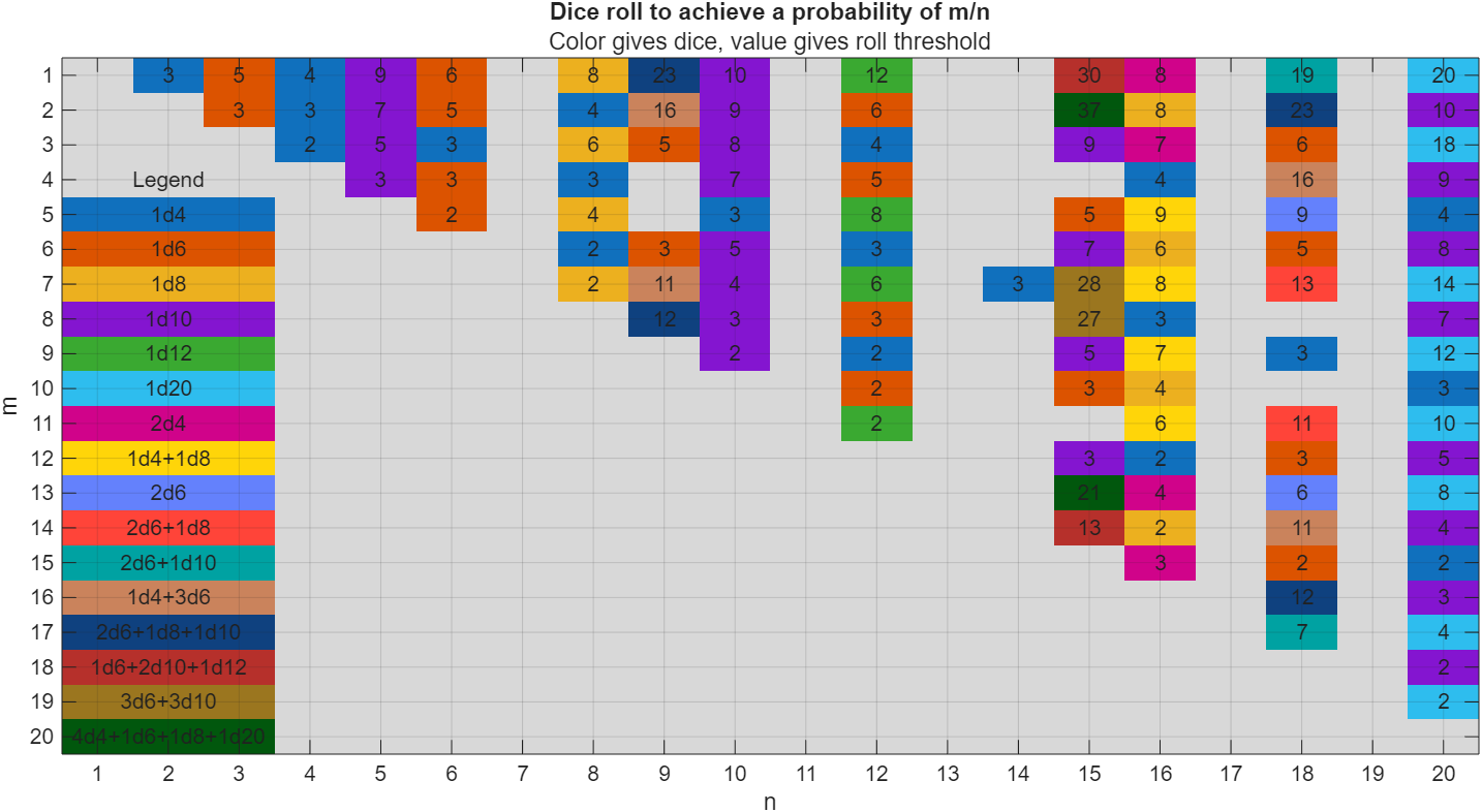
In the original xkcd, the situation described by the player has a probability of 2/9. Looking up the plot, row 2 column 9, shows that you need 16 or greater on (from the legend) 1d4+3d6, just as claimed.
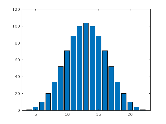
If you missed the bit about convolutions, this is a super-neat trick
[v,c] = dicedist([4 6 6 6]);
bar(v,c)
% Probability distribution of dice given by d
function [vals,counts] = dicedist(d)
% d is a vector of number of sides
n = numel(d); % number of dice
% Use convolution to count the number of ways to get each roll value
counts = 1;
for k = 1:n
counts = conv(counts,ones(1,d(k)));
end
% Possible values range from n to sum(d)
maxtot = sum(d);
vals = n:maxtot;
end
The pdist function allows the user to specify the function coding the similarity between rows of matrices (called DISTFUN in the documentation).
With the increasing diffusion of large datasets, techniques to sparsify graphs are increasingly being explored and used in practical applications. It is easy to code one own's DISTFUN such that it returns a sparse vector. Unfortunately, pdist (and pdist2) will return a dense vector in the output, which for very large graphs will cause an out of memory error. The offending code is
(lines 434 etc.)
% Make the return have whichever numeric type the distance function
% returns, or logical.
if islogical(Y)
Y = false(1,n*(n-1)./2);
else % isnumeric
Y = zeros(1,n*(n-1)./2, class(Y));
end
To have pdist return a sparse vector, the only modification that is required is
if islogical(Y)
Y = false(1,n*(n-1)./2);
elseif issparse(Y)
Y = sparse(1,n*(n-1)./2);
else % isnumeric
Y = zeros(1,n*(n-1)./2, class(Y));
end
It is a bit more work to modify squareform to produce a sparse matrix, given a sparse vector produced by the modified pdist. Squareform includes several checks on the inputs, but the core functionality for sparse vectors would be given by something like
% given a sparse vector d returned by pdist, compute a sparse squareform
[~,j,v] = find(d);
[m,n] = pdist_ind2sub(j, nobs);
W = sparse(m, n, v, nobs, nobs);
W = W + W';
Here, pdist_ind2sub is a function that given a set of indices into a vector produced by pdist, returns the corresponding subscripts in a (triangular) matrix. Computing this requires information about the number of observations given to pdist, i.e. what was n in the preceding code. I could not figure out a way to use the function adjacency to accomplish this.
MATLAB FEX(MATLAB File Exchange) should support Markdown syntax for writing. In recent years, many open-source community documentation platforms, such as GitHub, have generally supported Markdown. MATLAB is also gradually improving its support for Markdown syntax. However, when directly uploading files to the MATLAB FEX community and preparing to write an overview, the outdated document format buttons are still present. Even when directly uploading a Markdown document, it cannot be rendered. We hope the community can support Markdown syntax!
BTW,I know that open-source Markdown writing on GitHub and linking to MATLAB FEX is feasible, but this is a workaround. It would be even better if direct native support were available.
I am very pleased to share my book, with coauthors Professor Richard Davis and Associate Professor Sam Toan, titled "Chemical Engineering Analysis and Optimization Using MATLAB" published by Wiley: https://www.wiley.com/en-us/Chemical+Engineering+Analysis+and+Optimization+Using+MATLAB-p-9781394205363
Also in The MathWorks Book Program:
Chemical Engineering Analysis and Optimization Using MATLAB® introduces cutting-edge, highly in-demand skills in computer-aided design and optimization. With a focus on chemical engineering analysis, the book uses the MATLAB platform to develop reader skills in programming, modeling, and more. It provides an overview of some of the most essential tools in modern engineering design.
Chemical Engineering Analysis and Optimization Using MATLAB® readers will also find:
- Case studies for developing specific skills in MATLAB and beyond
- Examples of code both within the text and on a companion website
- End-of-chapter problems with an accompanying solutions manual for instructors
This textbook is ideal for advanced undergraduate and graduate students in chemical engineering and related disciplines, as well as professionals with backgrounds in engineering design.
My following code works running Matlab 2024b for all test cases. However, 3 of 7 tests fail (#1, #4, & #5) the QWERTY Shift Encoder problem. Any ideas what I am missing?
Thanks in advance.
keyboardMap1 = {'qwertyuiop[;'; 'asdfghjkl;'; 'zxcvbnm,'};
keyboardMap2 = {'QWERTYUIOP{'; 'ASDFGHJKL:'; 'ZXCVBNM<'};
if length(s) == 0
se = s;
end
for i = 1:length(s)
if double(s(i)) >= 65 && s(i) <= 90
row = 1;
col = 1;
while ~strcmp(s(i), keyboardMap2{row}(col))
if col < length(keyboardMap2{row})
col = col + 1;
else
row = row + 1;
col = 1;
end
end
se(i) = keyboardMap2{row}(col + 1);
elseif double(s(i)) >= 97 && s(i) <= 122
row = 1;
col = 1;
while ~strcmp(s(i), keyboardMap1{row}(col))
if col < length(keyboardMap1{row})
col = col + 1;
else
row = row + 1;
col = 1;
end
end
se(i) = keyboardMap1{row}(col + 1);
else
se(i) = s(i);
end
% if ~(s(i) = 65 && s(i) <= 90) && ~(s(i) >= 97 && s(i) <= 122)
% se(i) = s(i);
% end
end
Too small
22%
Just right
38%
Too large
40%
2648 votes
In one of my MATLAB projects, I want to add a button to an existing axes toolbar. The function for doing this is axtoolbarbtn:
axtoolbarbtn(tb,style,Name=Value)
However, I have found that the existing interfaces and behavior make it quite awkward to accomplish this task.
Here are my observations.
Adding a Button to the Default Axes Toolbar Is Unsupported
plot(1:10)
ax = gca;
tb = ax.Toolbar
Calling axtoolbarbtn on ax results in an error:
>> axtoolbarbtn(tb,"state")
Error using axtoolbarbtn (line 77)
Modifying the default axes toolbar is not supported.
Default Axes Toolbar Can't Be Distinguished from an Empty Toolbar
The Children property of the default axes toolbar is empty. Thus, it appears programmatically to have no buttons, just like an empty toolbar created by axtoolbar.
cla
plot(1:10)
ax = gca;
tb = ax.Toolbar;
tb.Children
ans = 0x0 empty GraphicsPlaceholder array.
tb2 = axtoolbar(ax);
tb2.Children
ans = 0x0 empty GraphicsPlaceholder array.
A Workaround
An empty axes toolbar seems to have no use except to initalize a toolbar before immediately adding buttons to it. Therefore, it seems reasonable to assume that an axes toolbar that appears to be empty is really the default toolbar. While we can't add buttons to the default axes toolbar, we can create a new toolbar that has all the same buttons as the default one, using axtoolbar("default"). And then we can add buttons to the new toolbar.
That observation leads to this workaround:
tb = ax.Toolbar;
if isempty(tb.Children)
% Assume tb is the default axes toolbar. Recreate
% it with the default buttons so that we can add a new
% button.
tb = axtoolbar(ax,"default");
end
btn = axtoolbarbtn(tb);
% Then set up the button as desired (icon, callback,
% etc.) by setting its properties.
As workarounds go, it's not horrible. It just seems a shame to have to delete and then recreate a toolbar just to be able to add a button to it.
The worst part about the workaround is that it is so not obvious. It took me a long time of experimentation to figure it out, including briefly giving it up as seemingly impossible.
The documentation for axtoolbarbtn avoids the issue. The most obvious example to write for axtoolbarbtn would be the first thing every user of it will try: add a toolbar button to the toolbar that gets created automatically in every call to plot. The doc page doesn't include that example, of course, because it wouldn't work.
My Request
I like the axes toolbar concept and the axes interactivity that it promotes, and I think the programming interface design is mostly effective. My request to MathWorks is to modify this interface to smooth out the behavior discontinuity of the default axes toolbar, with an eye towards satisfying (and documenting) the general use case that I've described here.
One possible function design solution is to make the default axes toolbar look and behave like the toolbar created by axtoolbar("default"), so that it has Children and so it is modifiable.
I am curious as to how my goal can be accomplished in Matlab.
The present APP called "Matching Network Designer" works quite well, but it is limited to a single section of a "PI", a "TEE", or an "L" topology circuit.
This limits the bandwidth capability of the APP when the intended use is to create an amplifier design intended for wider bandwidth projects.
I am requesting that a "Broadband Matching Network Designer" APP be developed by you, the MathWorks support team.
One suggestion from me is to be able to cascade a second section (or "pole") to the first.
Then the resulting topology would be capable of achieving that wider bandwidth of the microwave amplifier project where it would be later used with the transistor output and input matching networks.
Instead of limiting the APP to a single frequency, the entire s parameter file would be used as an input.
The APP would convert the polar s parameters to rectangular scaler complex impedances that you already use.
At that point, having started out with the first initial center frequency, the other frequencies both greater than and less than the center would come into use by an optimization of the circuit elements.
I'm hoping that you will be able to take on this project.
I can include an attachment of such a Matching Network Designer APP that you presently have if you like.
That network is centered at 10 GHz.
Kimberly Renee Alvarez.
310-367-5768
Overview
Authors:
- Narayanaswamy P.R. Iyer
- Provides Simulink models for various PWM techniques used for inverters
- Presents vector and direct torque control of inverter-fed AC drives and fuzzy logic control of converter-fed AC drives
- Includes examples, case studies, source codes of models, and model projects from all the chapters.
About this book
Successful development of power electronic converters and converter-fed electric drives involves system modeling, analyzing the output voltage, current, electromagnetic torque, and machine speed, and making necessary design changes before hardware implementation. Inverters and AC Drives: Control, Modeling, and Simulation Using Simulink offers readers Simulink models for single, multi-triangle carrier, selective harmonic elimination, and space vector PWM techniques for three-phase two-level, multi-level (including modular multi-level), Z-source, Quasi Z-source, switched inductor, switched capacitor and diode assisted extended boost inverters, six-step inverter-fed permanent magnet synchronous motor (PMSM), brushless DC motor (BLDCM) and induction motor (IM) drives, vector-controlled PMSM, IM drives, direct torque-controlled inverter-fed IM drives, and fuzzy logic controlled converter-fed AC drives with several examples and case studies. Appendices in the book include source codes for all relevant models, model projects, and answers to selected model projects from all chapters.
This textbook will be a valuable resource for upper-level undergraduate and graduate students in electrical and electronics engineering, power electronics, and AC drives. It is also a hands-on reference for practicing engineers and researchers in these areas.
I want to share a new book "Introduction to Digital Control - An Integrated Approach, Springer, 2024" available through https://link.springer.com/book/10.1007/978-3-031-66830-2.
This textbook presents an integrated approach to digital (discrete-time) control systems covering analysis, design, simulation, and real-time implementation through relevant hardware and software platforms. Topics related to discrete-time control systems include z-transform, inverse z-transform, sampling and reconstruction, open- and closed-loop system characteristics, steady-state accuracy for different system types and input functions, stability analysis in z-domain-Jury’s test, bilinear transformation from z- to w-domain, stability analysis in w-domain- Routh-Hurwitz criterion, root locus techniques in z-domain, frequency domain analysis in w-domain, control system specifications in time- and frequency- domains, design of controllers – PI, PD, PID, phase-lag, phase-lead, phase-lag-lead using time- and frequency-domain specifications, state-space methods- controllability and observability, pole placement controllers, design of observers (estimators) - full-order prediction, reduced-order, and current observers, system identification, optimal control- linear quadratic regulator (LQR), linear quadratic Gaussian (LQG) estimator (Kalman filter), implementation of controllers, and laboratory experiments for validation of analysis and design techniques on real laboratory scale hardware modules. Both single-input single-output (SISO) and multi-input multi-output (MIMO) systems are covered. Software platform of MATLAB/Simlink is used for analysis, design, and simulation and hardware/software platforms of National Instruments (NI)/LabVIEW are used for implementation and validation of analysis and design of digital control systems. Demonstrating the use of an integrated approach to cover interdisciplinary topics of digital control, emphasizing theoretical background, validation through analysis, simulation, and implementation in physical laboratory experiments, the book is ideal for students of engineering and applied science across in a range of concentrations.
I am excited to share my new book "Introduction to Mechatronics - An Integrated Approach, Springer, 2023" available through https://link.springer.com/book/10.1007/978-3-031-29320-7.
This textbook presents mechatronics through an integrated approach covering instrumentation, circuits and electronics, computer-based data acquisition and analysis, analog and digital signal processing, sensors, actuators, digital logic circuits, microcontroller programming and interfacing. The use of computer programming is emphasized throughout the text, and includes MATLAB for system modeling, simulation, and analysis; LabVIEW for data acquisition and signal processing; and C++ for Arduino-based microcontroller programming and interfacing. The book provides numerous examples along with appropriate program codes, for simulation and analysis, that are discussed in detail to illustrate the concepts covered in each section. The book also includes the illustration of theoretical concepts through the virtual simulation platform Tinkercad to provide students virtual lab experience.
I had originally planned on publishing my book via a traditional publisher, but am now reconsidering whether to use Amazon.com. I use Matlab and Latex in my book. It appears that it is not possible to publish is with Amazon due to this. Advice? Thanks. Kevin Passino
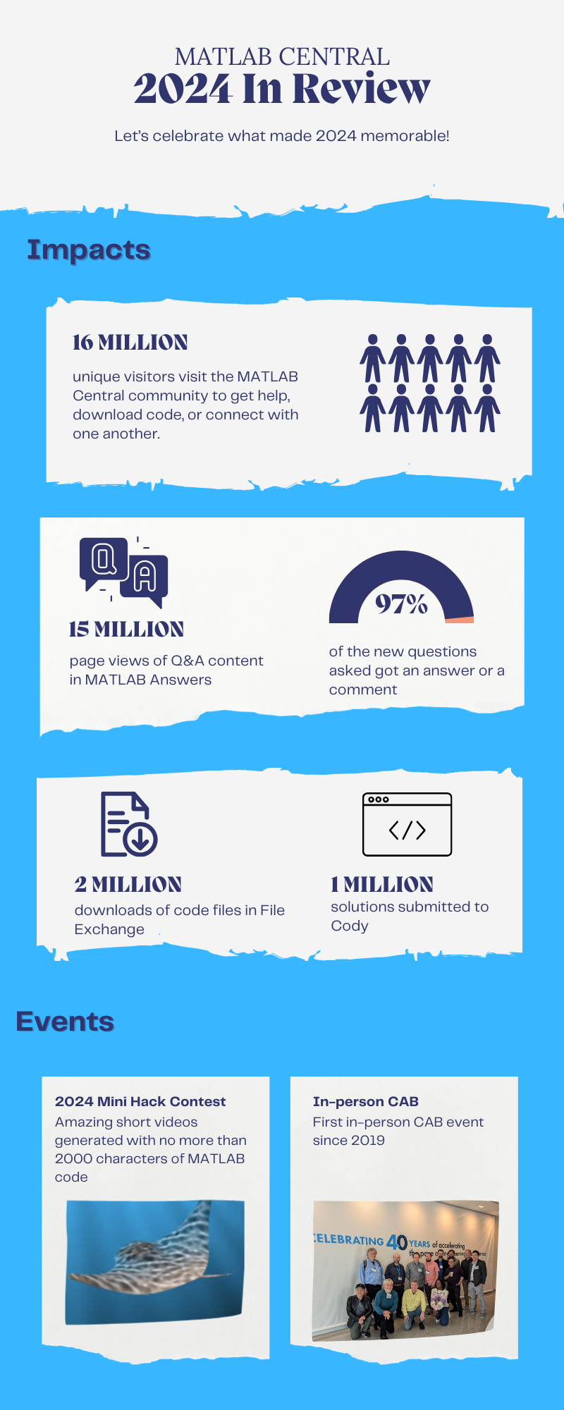
Let's celebrate what made 2024 memorable! Together, we made big impacts, hosted exciting events, and built new apps.

Resource links:
I have a skeleton and i want to find the start and end point of that skeleton. My skeleton is like an oval/donut where there is little gap between the start and end
Hello,
Now that the "Copilot+PC" (Windows ARM) laptops are rapidly increasing in market share (Microsoft Surface Laptop, Dell XPS 13, HP OmniBook X 14, and more), are there any plans to provide builds for Matlab on Windows arm64?
Since there are already Windows builds of Matlab, it shouldn't be too hard to compile for Windows arm64, as far as I know. But I am not famaliar with Matlab's codebase.
Please try to publish Windows arm64 builds soon so that Matlab can be much more usable on Windows on ARM as it will run natively instead of in emulation.
Thank you very much.
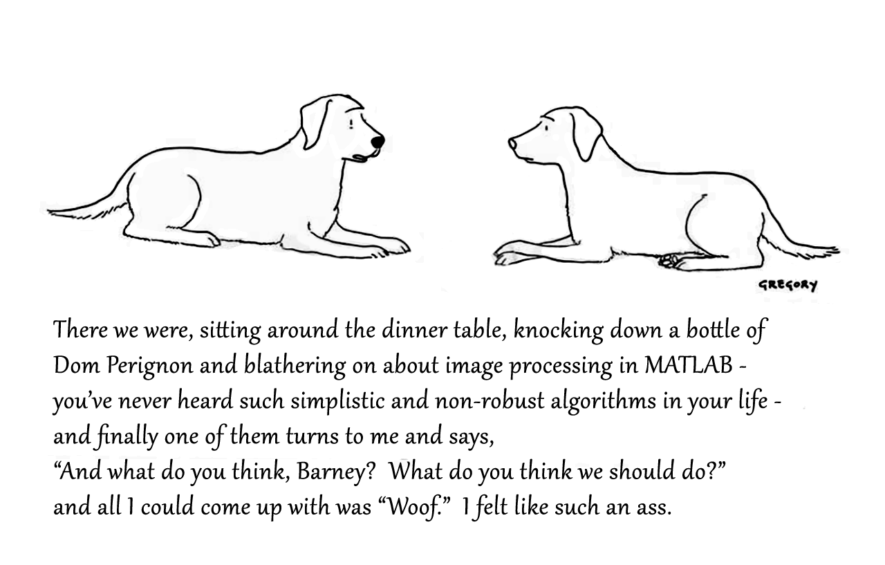
Attaching the Photoshop file if you want to modify the caption.
We’d like to announce a change on the Machine Translation feature on MATLAB Answers.
When users are visiting our international domains (e.g. China or Japan), Answers provides the option to translate the content. Recently, we identified several security threats involving high-volume requests from certain IP addresses targeting our translation service.
As one of the countermeasures, we have now placed the Machine Translation feature behind a login requirement. While non-logged-in users will still see the 'Translate' button, it will be inactive (greyed out) until they log in.
We are actively collaborating with adjacent teams to develop solutions to better detect and block malicious requests.
Please let us know if you have any questions or concerns.
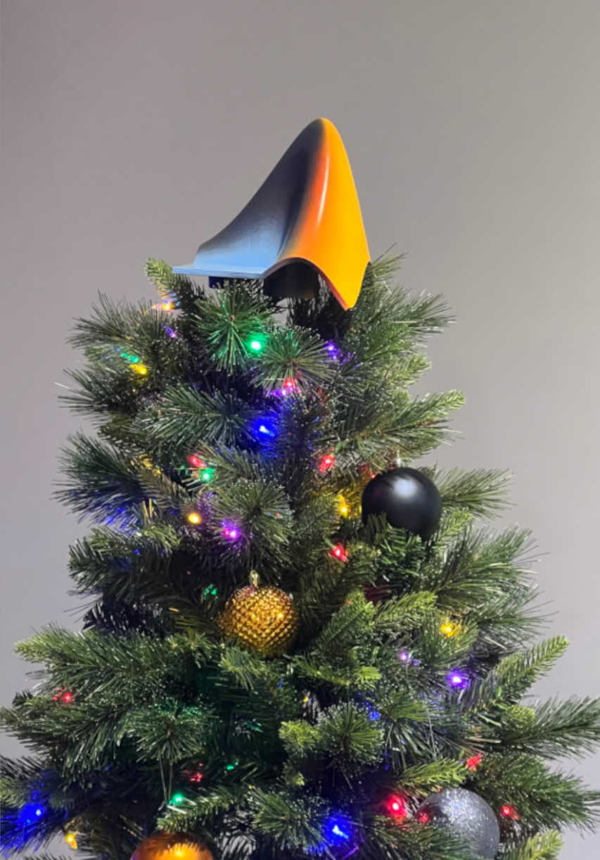
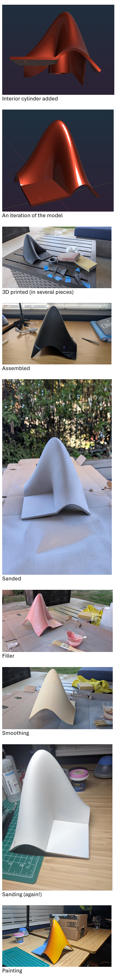
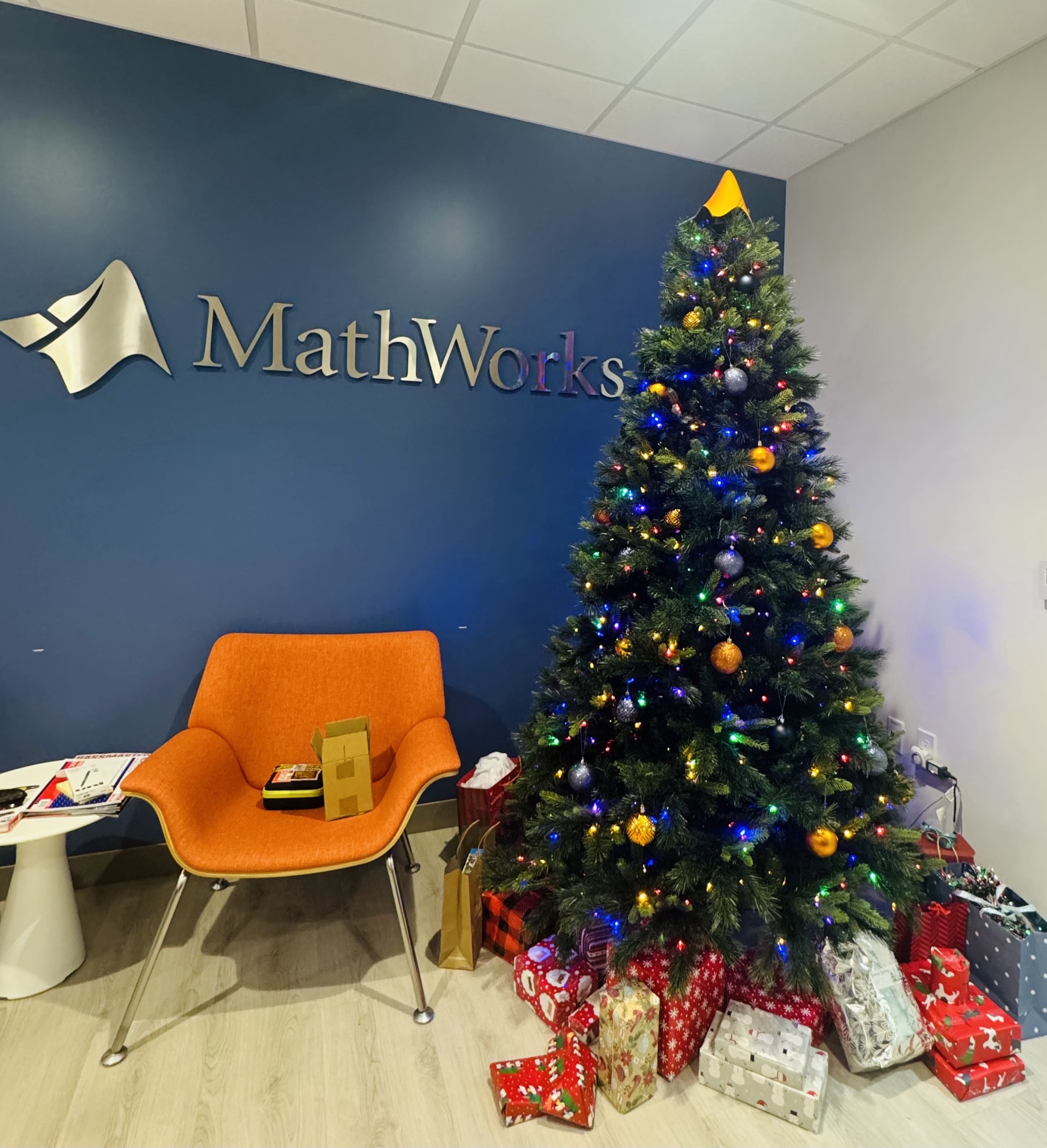
What better way to add a little holiday magic than the L-shaped membrane atop your evergreen? My colleagues output the shape and then added some thickness and an interior cylinder in Blender. Then, the shape was exported to STL and 3D printed (in several pieces). Then glued, sanded, primed, sanded again and painted. If you like, the STL file is attached. Thank you to https://blogs.mathworks.com/community/2013/06/20/paul-prints-the-l-shaped-membrane/ and a tip of the hat to MATLAB Ornament. Happy Holidays!
I have a problem with the movement of a pawn by two fields in its first move does anyone have a suggestion for a solution
function chess_game()
% Funkcja główna inicjalizująca grę w szachy
% Inicjalizacja stanu gry
gameState = struct();
gameState.board = initialize_board();
gameState.currentPlayer = 'white';
gameState.selectedPiece = [];
% Utworzenie GUI
fig = figure('Name', 'Gra w Szachy', 'NumberTitle', 'off', 'MenuBar', 'none', 'UserData', gameState);
ax = axes('Parent', fig, 'Position', [0 0 1 1], 'XTick', [], 'YTick', []);
axis(ax, [0 8 0 8]);
hold on;
% Wyświetlenie planszy
draw_board(ax, gameState.board);
% Obsługa kliknięcia myszy
set(fig, 'WindowButtonDownFcn', @(src, event)on_click(ax, src));
end
function board = initialize_board()
% Inicjalizuje planszę z ustawieniem początkowym figur
board = {
'R', 'N', 'B', 'Q', 'K', 'B', 'N', 'R';
'P', 'P', 'P', 'P', 'P', 'P', 'P', 'P';
'', '', '', '', '', '', '', '';
'', '', '', '', '', '', '', '';
'', '', '', '', '', '', '', '';
'', '', '', '', '', '', '', '';
'p', 'p', 'p', 'p', 'p', 'p', 'p', 'p';
'r', 'n', 'b', 'q', 'k', 'b', 'n', 'r';
};
end
function draw_board(~, board)
% Rysuje szachownicę i figury
colors = [1 1 1; 0.8 0.8 0.8];
for row = 1:8
for col = 1:8
% Rysowanie pól
rectColor = colors(mod(row + col, 2) + 1, :);
rectangle('Position', [col-1, 8-row, 1, 1], 'FaceColor', rectColor, 'EdgeColor', 'k');
% Rysowanie figur
piece = board{row, col};
if ~isempty(piece)
text(col-0.5, 8-row+0.5, piece, 'HorizontalAlignment', 'center', ...
'FontSize', 20, 'FontWeight', 'bold');
end
end
end
end
function on_click(ax, fig)
% Funkcja obsługująca kliknięcia myszy
pos = get(ax, 'CurrentPoint');
x = floor(pos(1,1)) + 1; % Zaokrąglij współrzędne w poziomie i dopasuj do indeksów
y = 8 - floor(pos(1,2)); % Dopasuj współrzędne w pionie (odwrócenie osi Y)
% Pobranie stanu gry z figury
gameState = get(fig, 'UserData');
if x >= 1 && x <= 8 && y >= 1 && y <= 8
disp(['Kliknięto na pole: (', num2str(x), ', ', num2str(y), ')']);
if isempty(gameState.selectedPiece)
% Wybór figury
piece = gameState.board{y, x};
if ~isempty(piece)
if (strcmp(gameState.currentPlayer, 'white') && any(ismember(piece, 'RNBQKP'))) || ...
(strcmp(gameState.currentPlayer, 'black') && any(ismember(piece, 'rnbqkp')))
gameState.selectedPiece = [y, x];
disp(['Wybrano figurę: ', piece, ' na pozycji (', num2str(x), ', ', num2str(y), ')']);
else
disp('Nie możesz wybrać tej figury.');
end
else
disp('Nie wybrano figury.');
end
else
% Sprawdzenie, czy kliknięto ponownie na wybraną figurę
if isequal(gameState.selectedPiece, [y, x])
disp('Anulowano wybór figury.');
gameState.selectedPiece = [];
else
% Ruch figury
[sy, sx] = deal(gameState.selectedPiece(1), gameState.selectedPiece(2));
piece = gameState.board{sy, sx};
if is_valid_move(gameState.board, piece, [sy, sx], [y, x], gameState.currentPlayer)
% Wykonanie ruchu
gameState.board{sy, sx} = ''; % Usuwamy figurę z poprzedniego pola
gameState.board{y, x} = piece; % Umieszczamy figurę na nowym polu
gameState.selectedPiece = [];
% Przełącz gracza
gameState.currentPlayer = switch_player(gameState.currentPlayer);
% Odśwież planszę
cla(ax);
draw_board(ax, gameState.board);
else
disp('Ruch niezgodny z zasadami.');
end
end
end
% Zaktualizowanie stanu gry w figurze
set(fig, 'UserData', gameState);
end
end
function valid = is_valid_move(board, piece, from, to, currentPlayer)
% Funkcja sprawdzająca, czy ruch jest poprawny
[sy, sx] = deal(from(1), from(2));
[dy, dx] = deal(to(1), to(2));
dy_diff = dy - sy;
dx_diff = abs(dx - sx);
targetPiece = board{dy, dx};
% Sprawdzenie, czy ruch jest w granicach planszy
if dx < 1 || dx > 8 || dy < 1 || dy > 8
valid = false;
return;
end
% Nie można zbijać swoich figur
if ~isempty(targetPiece) && ...
((strcmp(currentPlayer, 'white') && ismember(targetPiece, 'RNBQKP')) || ...
(strcmp(currentPlayer, 'black') && ismember(targetPiece, 'rnbqkp')))
valid = false;
return;
end
% Zasady ruchu dla każdej figury
switch lower(piece)
case 'p' % Pion
direction = strcmp(currentPlayer, 'white') * 2 - 1; % 1 dla białych, -1 dla czarnych
startRow = strcmp(currentPlayer, 'white') * 2 + 1; % Rząd startowy dla białych i czarnych
if isempty(targetPiece)
% Ruch o jedno pole do przodu
if dy_diff == direction && dx_diff == 0
valid = true;
% Ruch o dwa pola do przodu z pozycji startowej
elseif dy_diff == 2 * direction && dx_diff == 0 && sy == startRow
if isempty(board{sy + direction, sx}) && isempty(board{dy, dx})
valid = true;
else
valid = false;
end
else
valid = false;
end
else
% Zbijanie na ukos
valid = (dx_diff == 1) && (dy_diff == direction);
end
case 'r' % Wieża
valid = (dx_diff == 0 || dy_diff == 0) && path_is_clear(board, from, to);
case 'n' % Skoczek
valid = (dx_diff == 2 && abs(dy_diff) == 1) || (dx_diff == 1 && abs(dy_diff) == 2);
case 'b' % Goniec
valid = (dx_diff == abs(dy_diff)) && path_is_clear(board, from, to);
case 'q' % Hetman
valid = ((dx_diff == 0 || dy_diff == 0) || (dx_diff == abs(dy_diff))) && path_is_clear(board, from, to);
case 'k' % Król
valid = max(abs(dx_diff), abs(dy_diff)) == 1;
otherwise
valid = false;
end
end
function clear = path_is_clear(board, from, to)
% Sprawdza, czy ścieżka między polami jest wolna od innych figur
[sy, sx] = deal(from(1), from(2));
[dy, dx] = deal(to(1), to(2));
stepY = sign(dy - sy);
stepX = sign(dx - sx);
y = sy + stepY;
x = sx + stepX;
while y ~= dy || x ~= dx
if ~isempty(board{y, x})
clear = false;
return;
end
y = y + stepY;
x = x + stepX;
end
clear = true;
end
function nextPlayer = switch_player(currentPlayer)
% Przełącza aktywnego gracza
if strcmp(currentPlayer, 'white')
nextPlayer = 'black';
else
nextPlayer = 'white';
end
end
Speaking as someone with 31+ years of experience developing and using imshow, I want to advocate for retiring and replacing it.
The function imshow has behaviors and defaults that were appropriate for the MATLAB and computer monitors of the 1990s, but which are not the best choice for most image display situations in today's MATLAB. Also, the 31 years have not been kind to the imshow code base. It is a glitchy, hard-to-maintain monster.
My new File Exchange function, imview, illustrates the kind of changes that I think should be made. The function imview is a much better MATLAB graphics citizen and produces higher quality image display by default, and it dispenses with the whole fraught business of trying to resize the containing figure. Although this is an initial release that does not yet support all the useful options that imshow does, it does enough that I am prepared to stop using imshow in my own work.
The Image Processing Toolbox team has just introduced in R2024b a new image viewer called imageshow, but that image viewer is created in a special-purpose window. It does not satisfy the need for an image display function that works well with the axes and figure objects of the traditional MATLAB graphics system.
I have published a blog post today that describes all this in more detail. I'd be interested to hear what other people think.
Note: Yes, I know there is an Image Processing Toolbox function called imview. That one is a stub for an old toolbox capability that was removed something like 15+ years ago. The only thing the toolbox imview function does now is call error. I have just submitted a support request to MathWorks to remove this old stub.