Happy Pi Day!
3.14 π Day has arrived, and this post provides some very cool pi implementations and complete MATLAB code.
Firstly, in order to obtain the first n decimal places of pi, we need to write the following code (to prevent inaccuracies, we need to take a few more tails and perform another operation of taking the first n decimal places when needed):
function Pi=getPi(n)
if nargin<1,n=3;end
Pi=char(vpa(sym(pi),n+10));
Pi=abs(Pi)-48;
Pi=Pi(3:n+2);
end
With this function to obtain the decimal places of pi, our visualization journey has begun~Step by step, from simple to complex~(Please try to use newer versions of MATLAB to run, at least R17b)
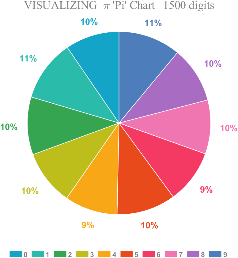
1 Pie chart
Just calculate the proportion of each digit to the first 1500 decimal places:
Pi=getPi(1500);
numNum=find([diff(sort(Pi)),1]);
numNum=[numNum(1),diff(numNum)];
CM=[20,164,199;43,187,170;53,165,81;189,190,28;248,167,22;
232,74,27;244,57,99;240,118,177;168,109,195;78,125,187]./255;
pieHdl=pie(numNum);
set(gcf,'Color',[1,1,1],'Position',[200,100,620,620]);
for i=1:2:20
pieHdl(i).EdgeColor=[1,1,1];
pieHdl(i).LineWidth=1;
pieHdl(i).FaceColor=CM((i+1)/2,:);
end
for i=2:2:20
pieHdl(i).Color=CM(i/2,:);
pieHdl(i).FontWeight='bold';
pieHdl(i).FontSize=14;
end
lgdHdl=legend(num2cell('0123456789'));
lgdHdl.FontWeight='bold';
lgdHdl.FontSize=11;
lgdHdl.TextColor=[.5,.5,.5];
lgdHdl.Location='southoutside';
lgdHdl.Box='off';
lgdHdl.NumColumns=10;
lgdHdl.ItemTokenSize=[20,15];
title("VISUALIZING \pi 'Pi' Chart | 1500 digits",'FontSize',18,...
'FontName','Times New Roman','Color',[.5,.5,.5])
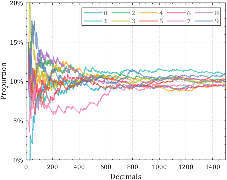
2 line chart
Calculate the change in the proportion of each number:
Pi=getPi(1500);
Ratio=cumsum(Pi==(0:9)',2);
Ratio=Ratio./sum(Ratio);
D=1:length(Ratio);
CM=[20,164,199;43,187,170;53,165,81;189,190,28;248,167,22;
232,74,27;244,57,99;240,118,177;168,109,195;78,125,187]./255;
hold on
for i=1:10
plot(D(20:end),Ratio(i,20:end),'Color',[CM(i,:),.6],'LineWidth',1.8)
end
ax=gca;box on;grid on
ax.YLim=[0,.2];
ax.YTick=0:.05:.2;
ax.XTick=0:200:1400;
ax.YTickLabel={'0%','5%','10%','15%','20%'};
ax.XMinorTick='on';
ax.YMinorTick='on';
ax.LineWidth=.8;
ax.GridLineStyle='-.';
ax.FontName='Cambria';
ax.FontSize=11;
ax.XLabel.String='Decimals';
ax.YLabel.String='Proportion';
ax.XLabel.FontSize=13;
ax.YLabel.FontSize=13;
lgdHdl=legend(num2cell('0123456789'));
lgdHdl.NumColumns=5;
lgdHdl.FontWeight='bold';
lgdHdl.FontSize=11;
lgdHdl.TextColor=[.5,.5,.5];
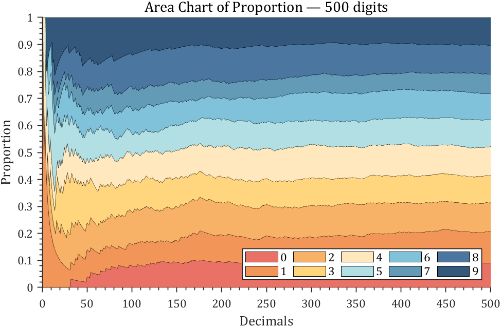
3 stacked area diagram
Pi=getPi(500);
Ratio=cumsum(Pi==(0:9)',2);
Ratio=Ratio./sum(Ratio);
CM=[231,98,84;239,138,71;247,170,88;255,208,111;255,230,183;
170,220,224;114,188,213;82,143,173;55,103,149;30,70,110]./255;
hold on
areaHdl=area(Ratio');
for i=1:10
areaHdl(i).FaceColor=CM(i,:);
areaHdl(i).FaceAlpha=.9;
end
set(gcf,'Position',[200,100,720,420]);
ax=gca;
ax.YLim=[0,1];
ax.XMinorTick='on';
ax.YMinorTick='on';
ax.LineWidth=.8;
ax.FontName='Cambria';
ax.FontSize=11;
ax.TickDir='out';
ax.XLabel.String='Decimals';
ax.YLabel.String='Proportion';
ax.XLabel.FontSize=13;
ax.YLabel.FontSize=13;
ax.Title.String='Area Chart of Proportion — 500 digits';
ax.Title.FontSize=14;
lgdHdl=legend(num2cell('0123456789'));
lgdHdl.NumColumns=5;
lgdHdl.FontSize=11;
lgdHdl.Location='southeast';
4 connected stacked bar chart
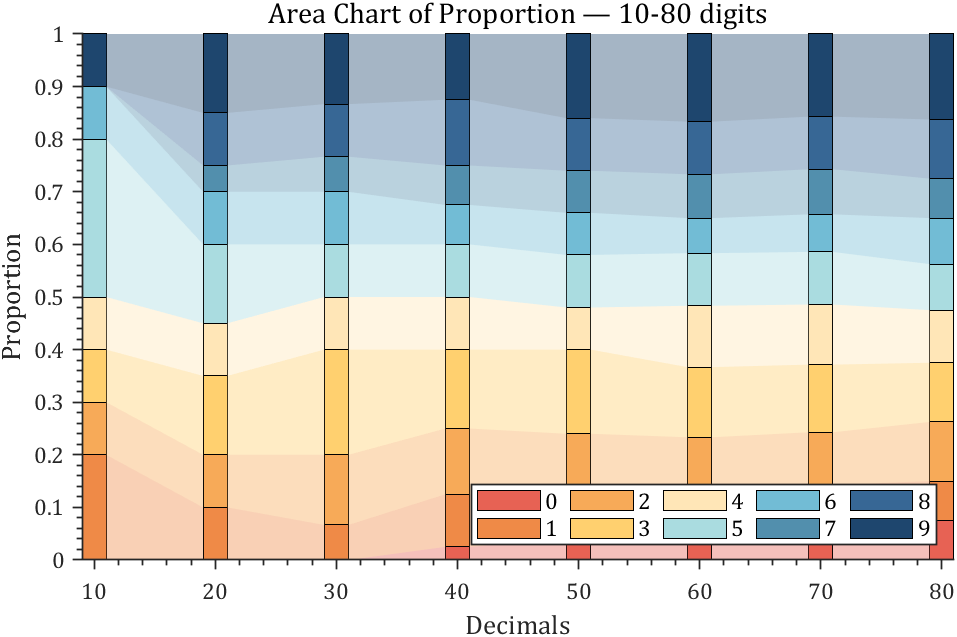
Pi=getPi(100);
Ratio=cumsum(Pi==(0:9)',2);
Ratio=Ratio./sum(Ratio);
X=Ratio(:,10:10:80)';
barHdl=bar(X,'stacked','BarWidth',.2);
CM=[231,98,84;239,138,71;247,170,88;255,208,111;255,230,183;
170,220,224;114,188,213;82,143,173;55,103,149;30,70,110]./255;
for i=1:10
barHdl(i).FaceColor=CM(i,:);
end
hold on;axis tight
yEndPoints=reshape([barHdl.YEndPoints]',length(barHdl(1).YData),[])';
zeros(1,length(barHdl(1).YData));
yEndPoints=[zeros(1,length(barHdl(1).YData));yEndPoints];
barWidth=barHdl(1).BarWidth;
for i=1:length(barHdl)
for j=1:length(barHdl(1).YData)-1
y1=min(yEndPoints(i,j),yEndPoints(i+1,j));
y2=max(yEndPoints(i,j),yEndPoints(i+1,j));
if y1*y2<0
ty=yEndPoints(find(yEndPoints(i+1,j)*yEndPoints(1:i,j)>=0,1,'last'),j);
y1=min(ty,yEndPoints(i+1,j));
y2=max(ty,yEndPoints(i+1,j));
end
y3=min(yEndPoints(i,j+1),yEndPoints(i+1,j+1));
y4=max(yEndPoints(i,j+1),yEndPoints(i+1,j+1));
if y3*y4<0
ty=yEndPoints(find(yEndPoints(i+1,j+1)*yEndPoints(1:i,j+1)>=0,1,'last'),j+1);
y3=min(ty,yEndPoints(i+1,j+1));
y4=max(ty,yEndPoints(i+1,j+1));
end
fill([j+.5.*barWidth,j+1-.5.*barWidth,j+1-.5.*barWidth,j+.5.*barWidth],...
[y1,y3,y4,y2],barHdl(i).FaceColor,'FaceAlpha',.4,'EdgeColor','none');
end
end
set(gcf,'Position',[200,100,720,420]);
ax=gca;box off
ax.YLim=[0,1];
ax.XMinorTick='on';
ax.YMinorTick='on';
ax.LineWidth=.8;
ax.FontName='Cambria';
ax.FontSize=11;
ax.TickDir='out';
ax.XTickLabel={'10','20','30','40','50','60','70','80'};
ax.XLabel.String='Decimals';
ax.YLabel.String='Proportion';
ax.XLabel.FontSize=13;
ax.YLabel.FontSize=13;
ax.Title.String='Area Chart of Proportion — 10-80 digits';
ax.Title.FontSize=14;
lgdHdl=legend(barHdl,num2cell('0123456789'));
lgdHdl.NumColumns=5;
lgdHdl.FontSize=11;
lgdHdl.Location='southeast';
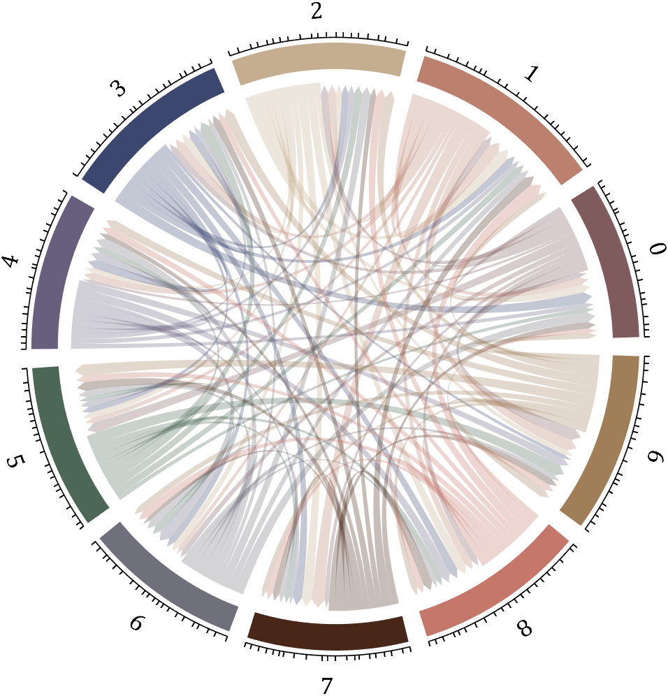
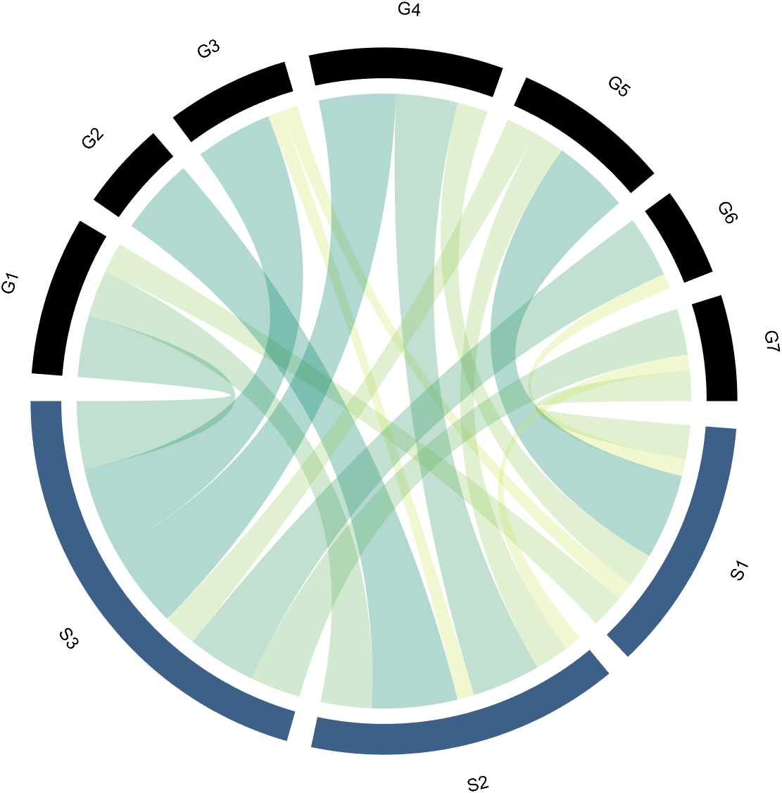
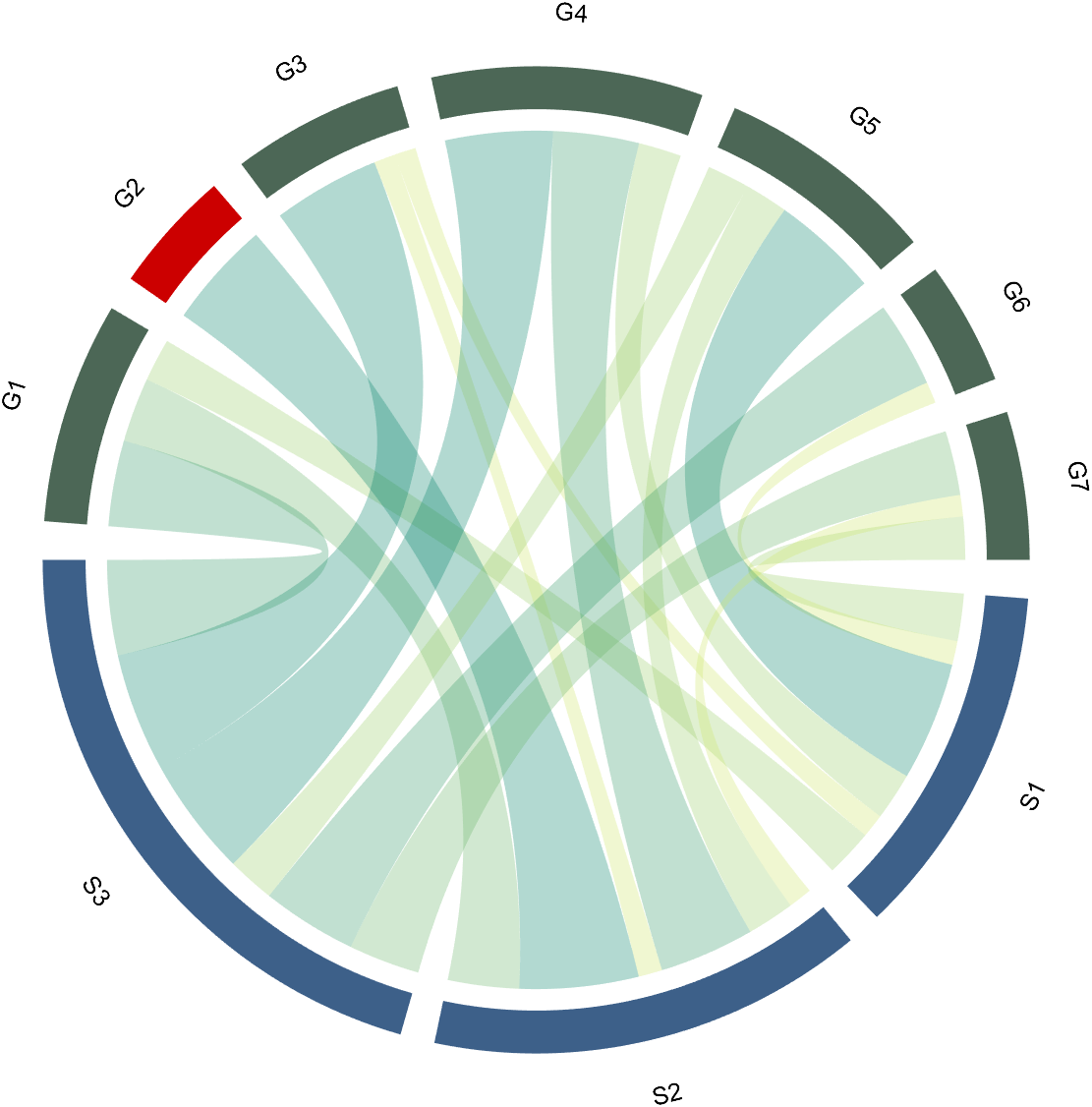
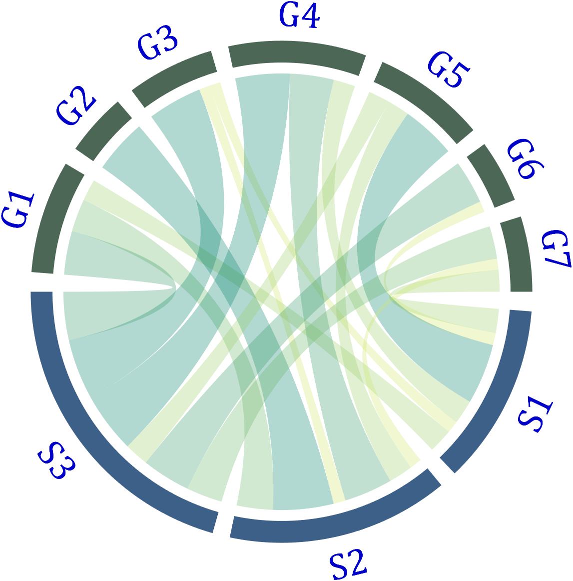
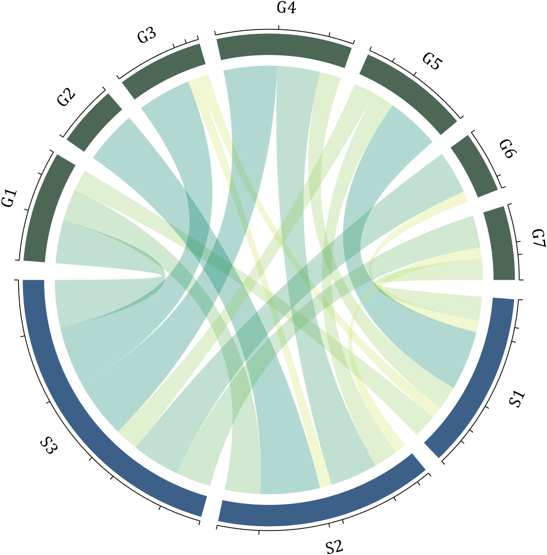
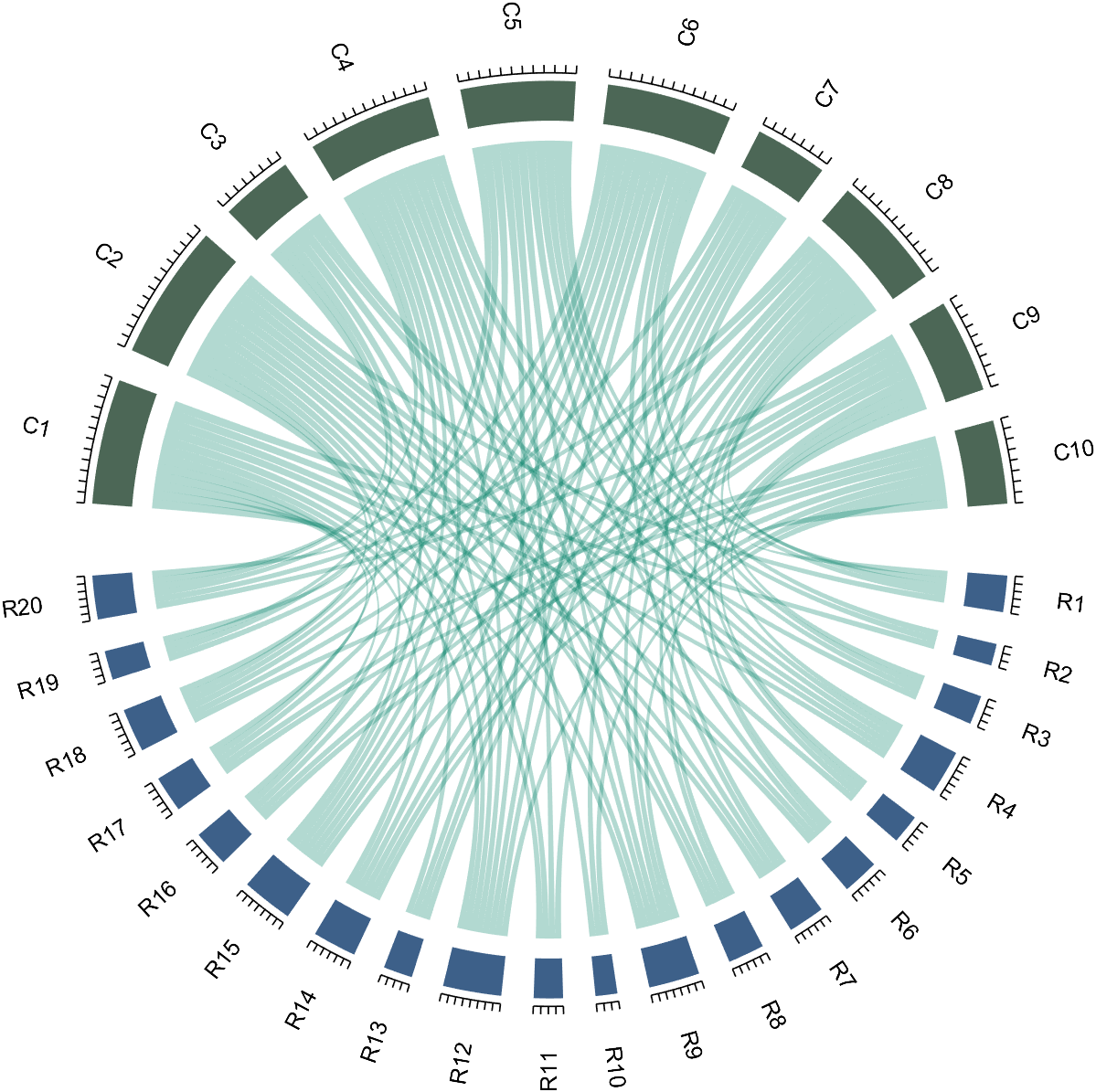
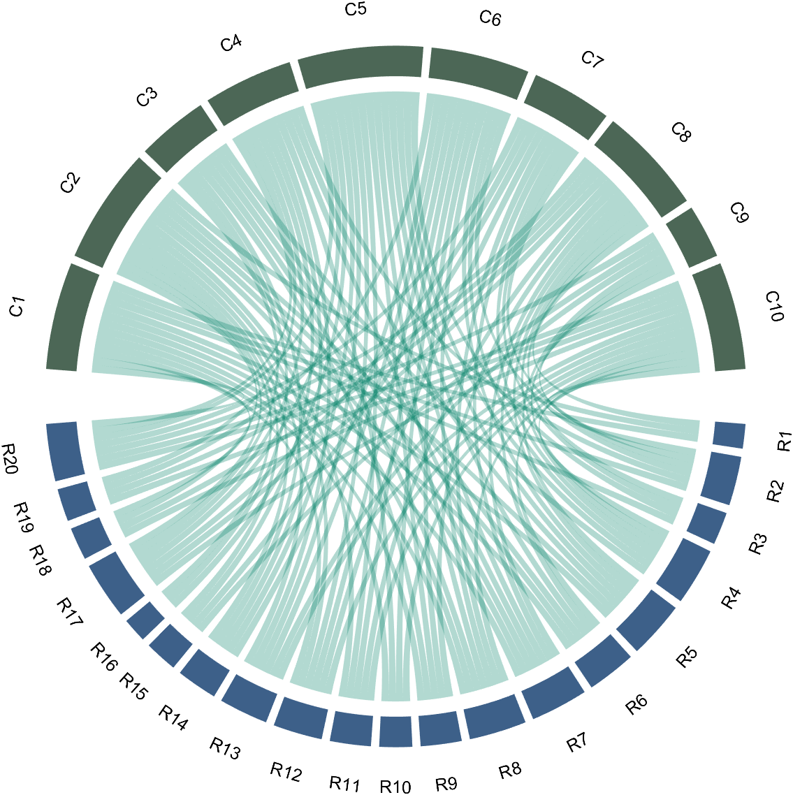
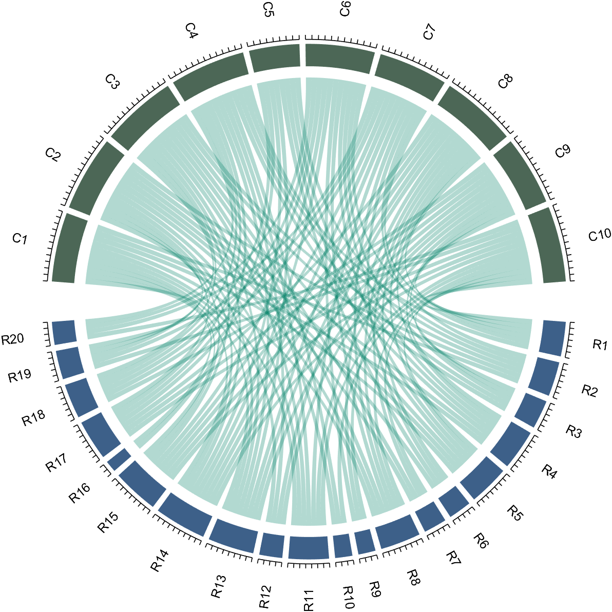
5 bichord chart
Need to use this tool:
dataMat=zeros(10,10);
Pi=getPi(1001);
for i=1:1000
dataMat(Pi(i)+1,Pi(i+1)+1)=dataMat(Pi(i)+1,Pi(i+1)+1)+1;
end
BCC=biChordChart(dataMat,'Arrow','on','Label',num2cell('0123456789'));
BCC=BCC.draw();
BCC.tickState('on')
BCC.setFont('FontName','Cambria','FontSize',17)
set(gcf,'Position',[200,100,820,820]);
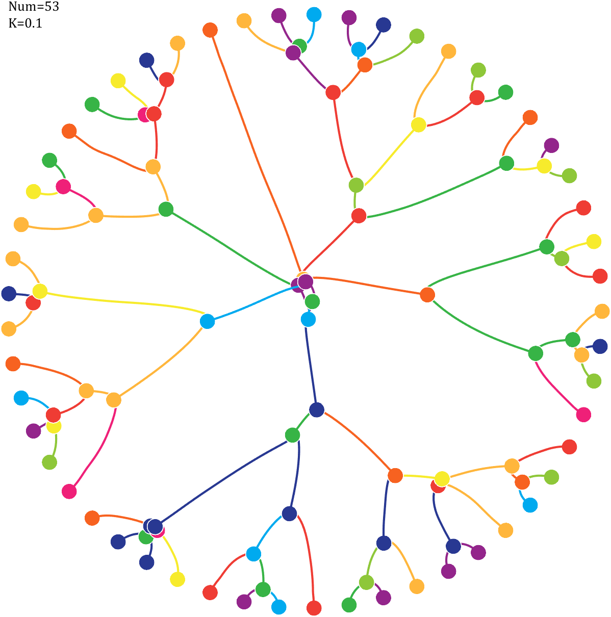
6 Gravity simulation diagram
Imagine each decimal as a small ball with a mass of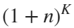
For example, if , the weight of ball 0 is 1, ball 9 is 1.2589, the initial velocity of the ball is 0, and it is attracted by other balls. Gravity follows the inverse square law, and if the balls are close enough, they will collide and their value will become
After adding, take the mod, add the velocity direction proportionally, and recalculate the weight.
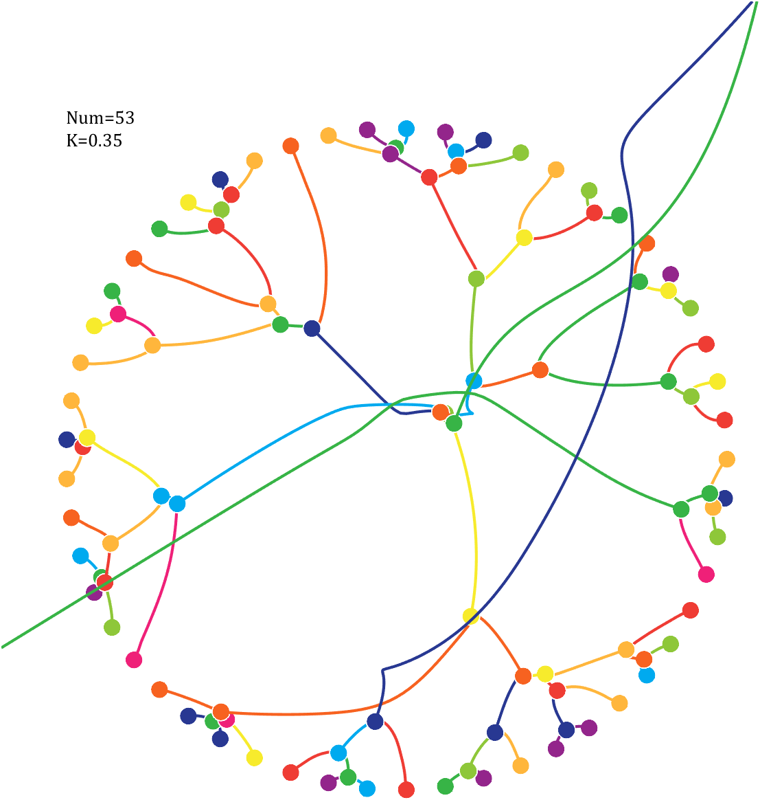
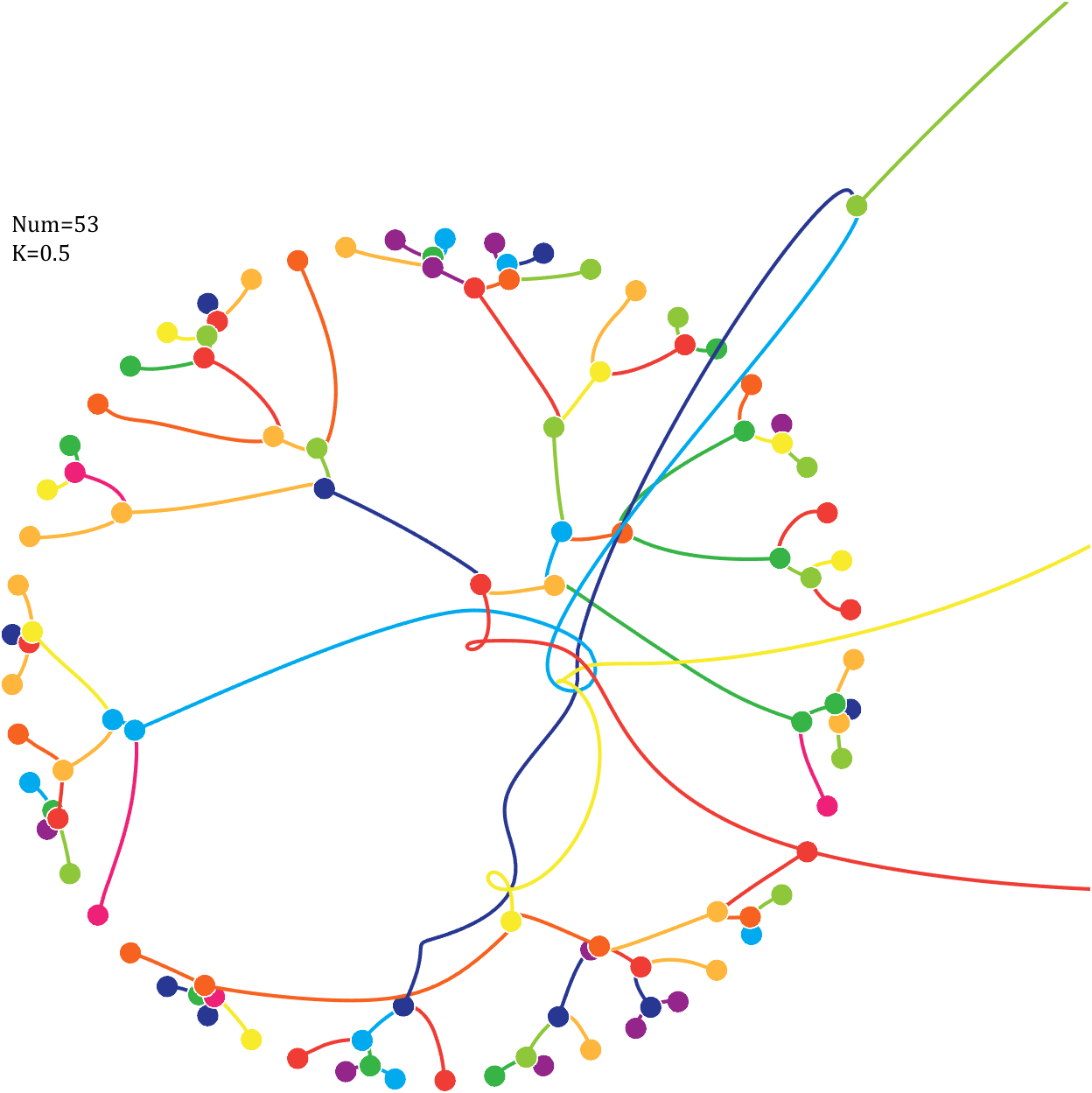
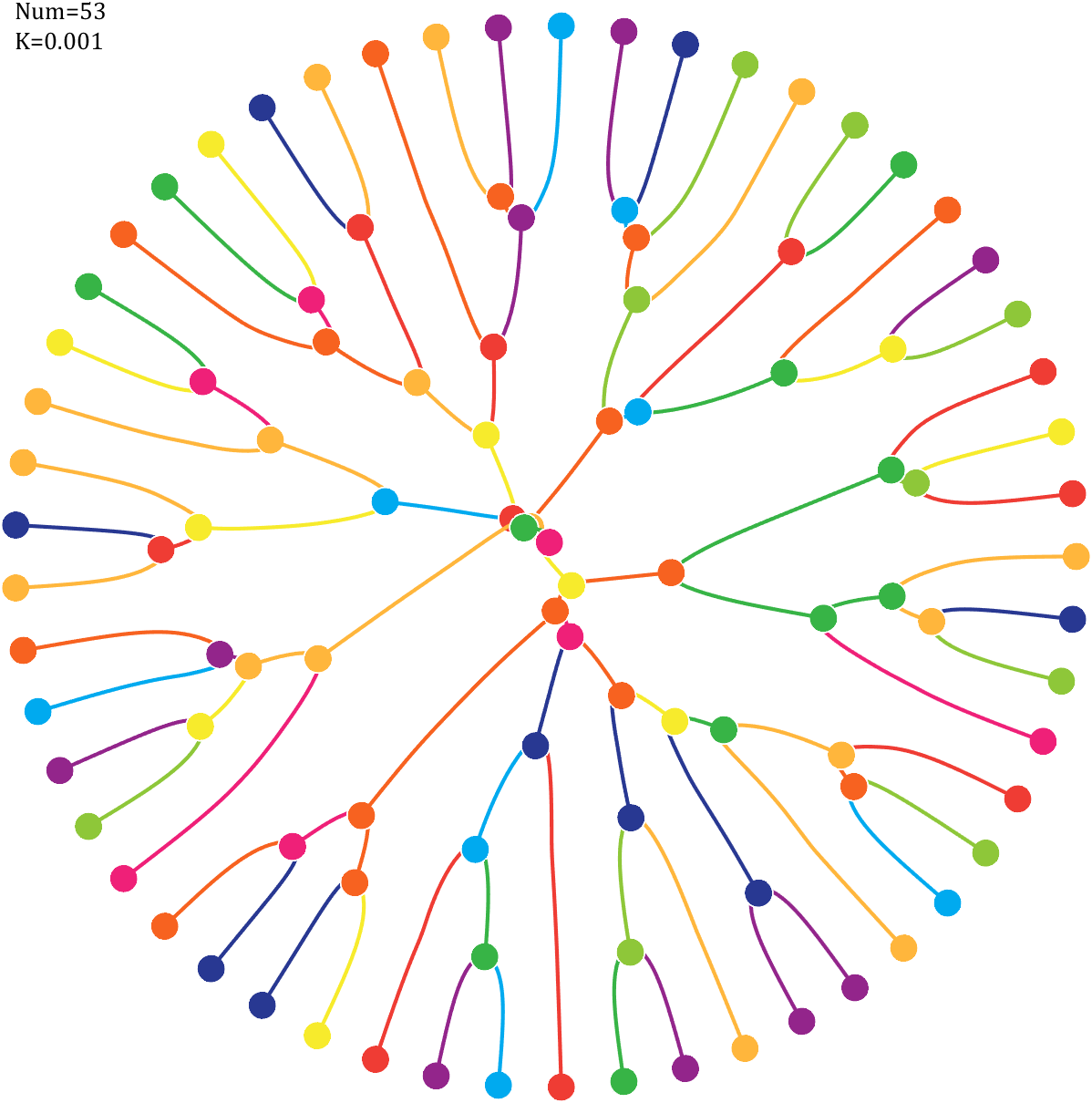
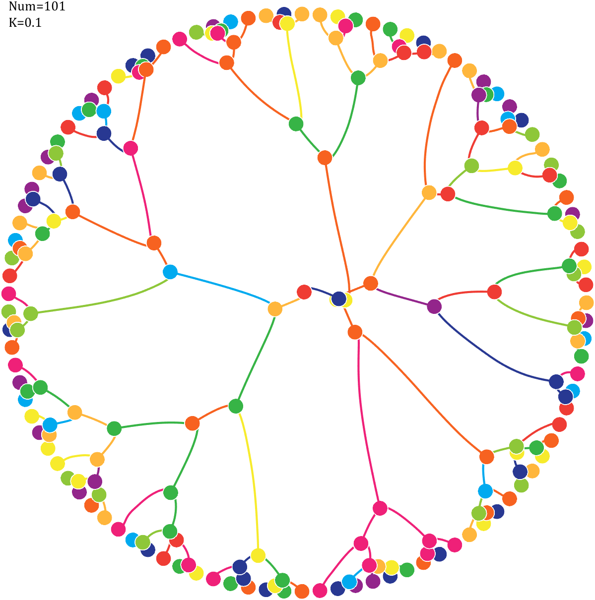
Pi=[3,getPi(71)];K=.18;
CM=[239,32,120;239,60,52;247,98,32;255,182,60;247,235,44;
142,199,57;55,180,70;0,170,239;40,56,146;147,37,139]./255;
T=linspace(0,2*pi,length(Pi)+1)';
T=T(1:end-1);
ct=linspace(0,2*pi,100);
cx=cos(ct).*.027;
cy=sin(ct).*.027;
Pi=Pi(:);
N=Pi;
X=cos(T);Y=sin(T);
VX=T.*0;VY=T.*0;
PX=X;PY=Y;
getM=@(x)(x+1).^K;
M=getM(N);
hold on
for i=1:length(N)
fill(cx+X(i),cy+Y(i),CM(N(i)+1,:),'EdgeColor','w','LineWidth',1)
end
for k=1:800
Rn2=1./squareform(pdist([X,Y])).^2;
Rn2(eye(length(X))==1)=0;
MRn2=Rn2.*(M');
AX=X'-X;AY=Y'-Y;
normXY=sqrt(AX.^2+AY.^2);
AX=AX./normXY;AX(eye(length(X))==1)=0;
AY=AY./normXY;AY(eye(length(X))==1)=0;
AX=sum(AX.*MRn2,2)./150000;
AY=sum(AY.*MRn2,2)./150000;
VX=VX+AX;X=X+VX;PX=[PX,X];
VY=VY+AY;Y=Y+VY;PY=[PY,Y];
R=squareform(pdist([X,Y]));
R(triu(ones(length(X)))==1)=inf;
[row,col]=find(R<=0.04);
if length(X)==1
break;
end
if ~isempty(row)
XC=(X(row)+X(col))./2;YC=(Y(row)+Y(col))./2;
VXC=(VX(row).*M(row)+VX(col).*M(col))./(M(row)+M(col));
VYC=(VY(row).*M(row)+VY(col).*M(col))./(M(row)+M(col));
PC=nan(length(row),size(PX,2));
NC=mod(N(row)+N(col),10);
uniNum=unique([row;col]);
X(uniNum)=[];VX(uniNum)=[];
Y(uniNum)=[];VY(uniNum)=[];
for i=1:length(uniNum)
plot(PX(uniNum(i),:),PY(uniNum(i),:),'LineWidth',2,'Color',CM(N(uniNum(i))+1,:))
end
PX(uniNum,:)=[];PY(uniNum,:)=[];N(uniNum,:)=[];
for i=1:length(XC)
fill(cx+XC(i),cy+YC(i),CM(NC(i)+1,:),'EdgeColor','w','LineWidth',1)
end
X=[X;XC];Y=[Y;YC];VX=[VX;VXC];VY=[VY;VYC];
PX=[PX;PC];PY=[PY;PC];N=[N;NC];M=getM(N);
end
end
for i=1:size(PX,1)
plot(PX(i,:),PY(i,:),'LineWidth',2,'Color',CM(N(i)+1,:))
end
text(-1,1,{['Num=',num2str(length(Pi))];['K=',num2str(K)]},'FontSize',13,'FontName','Cambria')
set(gcf,'Position',[200,100,820,820]);
ax=gca;
ax.Position=[0,0,1,1];
ax.DataAspectRatio=[1,1,1];
ax.XLim=[-1.1,1.1];
ax.YLim=[-1.1,1.1];
ax.XTick=[];
ax.YTick=[];
ax.XColor='none';
ax.YColor='none';
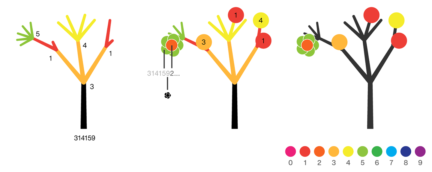
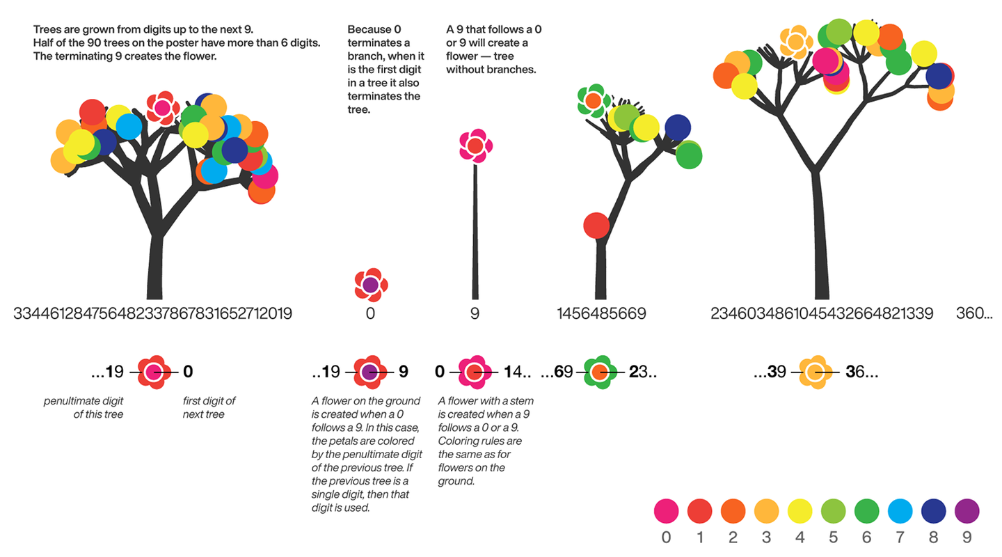
7 forest chart
The method comes from
The digits of π are shown as a forest. Each tree in the forest represents the digits of π up to the next 9. The first 10 trees are "grown" from the digit sets 314159, 2653589, 79, 3238462643383279, 50288419, 7169, 39, 9, 3751058209, and 749.
BRANCHES
The first digit of a tree controls how many branches grow from the trunk of the tree. For example, the first tree's first digit is 3, so you see 3 branches growing from the trunk.
The next digit's branches grow from the end of a branch of the previous digit in left-to-right order. This process continues until all the tree's digits have been used up.
Each tree grows from a set of consecutive digits sampled from the digits of π up to the next 9. The first tree, shown here, grows from 314159. Each of the digits determine how many branches grow at each fork in the tree — the branches here are colored by their corresponding digit to illustrate this. Leaves encode the digits in a left-to-right order. The digit 9 spawns a flower on one of the branches of the previous digit. The branching exception is 0, which terminates the current branch — 0 branches grow!
LEAVES AND FLOWERS
The tree's digits themselves are drawn as circular leaves, color-coded by the digit.
The leaf exception is 9, which causes one of the branches of the previous digit to sprout a flower! The petals of the flower are colored by the digit before the 9 and the center is colored by the digit after the 9, which is on the next tree. This is how the forest propagates.
The colors of a flower are determined by the first digit of the next tree and the penultimate digit of the current tree. If the current tree only has one digit, then that digit is used. Leaves are placed at the tips of branches in a left-to-right order — you can "easily" read them off. Additionally, the leaves are distributed within the tree (without disturbing their left-to-right order) to spread them out as much as possible and avoid overlap. This order is deterministic.
The leaf placement exception are the branch set that sprouted the flower. These are not used to grow leaves — the flower needs space!
function PiTree(X,pos,D)
lw=2;
theta=pi/2+(rand(1)-.5).*pi./12;
CM=[237,32,121;237,62,54;247,99,33;255,183,59;245,236,43;
141,196,63;57,178,74;0,171,238;40,56,145;146,39,139]./255;
hold on
if all(X(1:end-2)==0)
endSet=[pos,pos,theta];
else
kplot(pos(1)+[0,cos(theta)],pos(2)+[0,sin(theta)],lw./.6)
endSet=[pos,pos+[cos(theta),sin(theta)],theta];
Layer=0;
for i=1:length(X)
Layer=[Layer,ones(1,X(i)).*i];
end
if D
for i=1:length(X)-2
if X(i)==0
newSet=endSet(1,:);
elseif X(i)==1
tTheta=endSet(1,5);
tTheta=linspace(tTheta+pi/8,tTheta-pi/8,2)'+(rand([2,1])-.5).*pi./8;
newSet=repmat(endSet(1,3:4),[X(i),1]);
newSet=[newSet.*[1;1],newSet+[cos(tTheta),sin(tTheta)].*.7^Layer(i).*[1;.1],tTheta];
else
tTheta=endSet(1,5);
tTheta=linspace(tTheta+pi/5,tTheta-pi/5,X(i))'+(rand([X(i),1])-.5).*pi./8;
newSet=repmat(endSet(1,3:4),[X(i),1]);
newSet=[newSet,newSet+[cos(tTheta),sin(tTheta)].*.7^Layer(i),tTheta];
end
for j=1:size(newSet,1)
kplot(newSet(j,[1,3]),newSet(j,[2,4]),lw.*.6^Layer(i))
end
endSet=[endSet;newSet];
endSet(1,:)=[];
end
end
end
FLSet=endSet(:,3:4);
[~,FLInd]=sort(FLSet(:,1));
FLSet=FLSet(FLInd,:);
[~,tempInd]=sort(rand([1,size(FLSet,1)]));
tempInd=sort(tempInd(1:length(X)-2));
flowerInd=tempInd(randi([1,length(X)-2],[1,1]));
leafInd=tempInd(tempInd~=flowerInd);
for i=1:length(leafInd)
scatter(FLSet(leafInd(i),1),FLSet(leafInd(i),2),70,'filled','CData',CM(X(i)+1,:))
end
for i=1:5
scatter(FLSet(flowerInd,1)+cos(pi*2*i/5).*.18,FLSet(flowerInd,2)+sin(pi*2*i/5).*.18,60,...
'filled','CData',CM(X(end-2)+1,:),'MarkerEdgeColor',[1,1,1])
end
scatter(FLSet(flowerInd,1),FLSet(flowerInd,2),60,'filled','CData',CM(X(end)+1,:),'MarkerEdgeColor',[1,1,1])
drawnow;
function kplot(XX,YY,LW,varargin)
LW=linspace(LW,LW*.6,10);
XX=linspace(XX(1),XX(2),11)';
XX=[XX(1:end-1),XX(2:end)];
YY=linspace(YY(1),YY(2),11)';
YY=[YY(1:end-1),YY(2:end)];
for ii=1:10
plot(XX(ii,:),YY(ii,:),'LineWidth',LW(ii),'Color',[.1,.1,.1])
end
end
end
main part:
Pi=[3,getPi(800)];
pos9=[0,find(Pi==9)];
set(gcf,'Position',[200,50,900,900],'Color',[1,1,1]);
ax=gca;hold on
ax.Position=[0,0,1,1];
ax.DataAspectRatio=[1,1,1];
ax.XLim=[.5,36];
ax.XTick=[];
ax.YTick=[];
ax.XColor='none';
ax.YColor='none';
for j=1:8
for i=1:11
n=i+(j-1)*11;
if n<=85
tPi=Pi((pos9(n)+1):pos9(n+1)+1);
if length(tPi)>2
PiTree(tPi,[0+i*3,0-j*4],true);
else
PiTree([Pi(pos9(n)),tPi],[0+i*3,0-j*4],false);
end
end
end
end
8 random walk
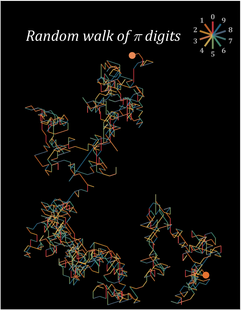
n=1200;
Pi=getPi(n);
CM=[239,65,75;230,115,48;229,158,57;232,136,85;239,199,97;
144,180,116;78,166,136;81,140,136;90,118,142;43,121,159]./255;
hold on
endPoint=[0,0];
t=linspace(0,2*pi,100);
T=linspace(0,2*pi,11)+pi/2;
fill(endPoint(1)+cos(t).*.5,endPoint(2)+sin(t).*.5,CM(Pi(1)+1,:),'EdgeColor','none')
for i=1:n
theta=T(Pi(i)+1);
plot(endPoint(1)+[0,cos(theta)],endPoint(2)+[0,sin(theta)],'Color',[CM(Pi(i)+1,:),.8],'LineWidth',1.2);
endPoint=endPoint+[cos(theta),sin(theta)];
end
fill(endPoint(1)+cos(t).*.5,endPoint(2)+sin(t).*.5,CM(Pi(n)+1,:),'EdgeColor','none')
set(gcf,'Position',[200,100,820,820]);
ax=gca;
ax.XTick=[];
ax.YTick=[];
ax.Color=[0,0,0];
ax.DataAspectRatio=[1,1,1];
ax.XLim=[-30,5];
ax.YLim=[-5,40];
endPoint=[1,35];
for i=1:10
theta=T(i);
plot(endPoint(1)+[0,cos(theta).*2],endPoint(2)+[0,sin(theta).*2],'Color',[CM(i,:),.8],'LineWidth',3);
text(endPoint(1)+cos(theta).*2.7,endPoint(2)+sin(theta).*2.7,num2str(i-1),'Color',[1,1,1].*.7,...
'FontSize',12,'FontWeight','bold','FontName','Cambria','HorizontalAlignment','center')
end
text(-15,35,'Random walk of \pi digits','Color',[1,1,1],'FontName','Cambria',...
'HorizontalAlignment','center','FontSize',25,'FontAngle','italic')
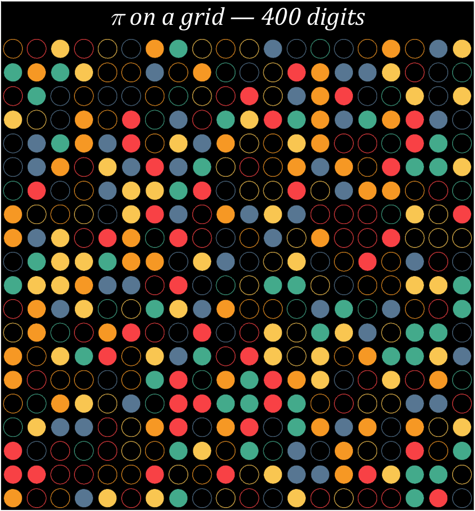
9 grid chart
Pi=[3,getPi(399)];
CM=[248,65,69;246,152,36;249,198,81;67,170,139;87,118,146]./255;
hold on
t=linspace(0,2*pi,100);
x=cos(t).*.8.*.5;
y=sin(t).*.8.*.5;
for i=1:400
[col,row]=ind2sub([20,20],i);
if mod(Pi(i),2)==0
fill(x+col,y+row,CM(round((Pi(i)+1)/2),:),'LineWidth',1,'EdgeAlpha',.8)
else
fill(x+col,y+row,[0,0,0],'EdgeColor',CM(round((Pi(i)+1)/2),:),'LineWidth',1,'EdgeAlpha',.7)
end
end
text(10.5,-.4,'\pi on a grid — 400 digits','Color',[1,1,1],'FontName','Cambria',...
'HorizontalAlignment','center','FontSize',25,'FontAngle','italic')
set(gcf,'Position',[200,100,820,820]);
ax=gca;
ax.YDir='reverse';
ax.XLim=[.5,20.5];
ax.YLim=[-1,20.5];
ax.XTick=[];
ax.YTick=[];
ax.Color=[0,0,0];
ax.DataAspectRatio=[1,1,1];
10 scale grid diagram
Let's still put the numbers in the form of circles, but the difference is that six numbers are grouped together, and the pure purple circle at the end is the six 9s that we are familiar with decimal places 762-767
Pi=[3,getPi(767)];
CM=[239,32,120;239,60,52;247,98,32;255,182,60;247,235,44;
142,199,57;55,180,70;0,170,239;40,56,146;147,37,139]./255;
hold on
t=linspace(0,2*pi,100);
x=cos(t).*.9.*.5;
y=sin(t).*.9.*.5;
for i=1:6:length(Pi)
n=round((i-1)/6+1);
[col,row]=ind2sub([10,13],n);
tNum=Pi(i:i+5);
numNum=find([diff(sort(tNum)),1]);
numNum=[numNum(1),diff(numNum)];
cumNum=cumsum(numNum);
uniNum=unique(tNum);
for j=length(cumNum):-1:1
fill(x./6.*cumNum(j)+col,y./6.*cumNum(j)+row,CM(uniNum(j)+1,:),'EdgeColor','none')
end
end
for i=1:10
fill(x./4+5.5+(i-5.5)*.32,y./4+14.5,CM(i,:),'EdgeColor','none')
text(5.5+(i-5.5)*.32,14.9,num2str(i-1),'Color',[1,1,1],'FontSize',...
9,'FontName','Cambria','HorizontalAlignment','center')
end
text(5.5,-.2,'FEYNMAN POINT of \pi','Color',[1,1,1],'FontName','Cambria',...
'HorizontalAlignment','center','FontSize',25,'FontAngle','italic')
set(gcf,'Position',[200,100,600,820]);
ax=gca;
ax.YDir='reverse';
ax.Position=[0,0,1,1];
ax.XLim=[.3,10.7];
ax.YLim=[-1,15.5];
ax.XTick=[];
ax.YTick=[];
ax.Color=[0,0,0];
ax.DataAspectRatio=[1,1,1];
11 text chart
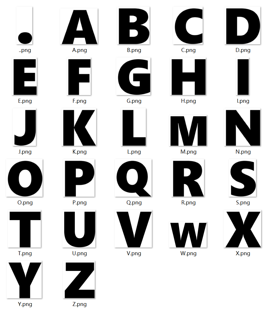
First, write a code to generate an image of each letter:
function getLogo
if ~exist('image','dir')
mkdir('image\')
end
logoSet=['.',char(65:90)];
for i=1:27
figure();
ax=gca;
ax.XLim=[-1,1];
ax.YLim=[-1,1];
ax.XColor='none';
ax.YColor='none';
ax.DataAspectRatio=[1,1,1];
logo=logoSet(i);
hold on
text(0,0,logo,'HorizontalAlignment','center','FontSize',320,'FontName','Segoe UI Black')
exportgraphics(ax,['image\',logo,'.png'])
close
end
dotPic=imread('image\..png');
newDotPic=uint8(ones([400,size(dotPic,2),3]).*255);
newDotPic(end-size(dotPic,1)+1:end,:,1)=dotPic(:,:,1);
newDotPic(end-size(dotPic,1)+1:end,:,2)=dotPic(:,:,2);
newDotPic(end-size(dotPic,1)+1:end,:,3)=dotPic(:,:,3);
imwrite(newDotPic,'image\..png')
S=20;
for i=1:27
logo=logoSet(i);
tPic=imread(['image\',logo,'.png']);
sz=size(tPic,[1,2]);
sz=round(sz./sz(1).*400);
tPic=imresize(tPic,sz);
tBox=uint8(255.*ones(size(tPic,[1,2])+S));
tBox(S+1:S+size(tPic,1),S+1:S+size(tPic,2))=tPic(:,:,1);
imwrite(cat(3,tBox,tBox,tBox),['image\',logo,'.png'])
end
end
Pi=[3,-1,getPi(150)];
CM=[109,110,113;224,25,33;244,126,26;253,207,2;154,203,57;111,150,124;
121,192,235;6,109,183;190,168,209;151,118,181;233,93,163]./255;
ST={'.','ZERO','ONE','TWO','THREE','FOUR','FIVE','SIX','SEVEN','EIGHT','NINE'};
n=1;
hold on
for i=1:20
STList='';
NMList=[];
PicListR=uint8(zeros(400,0));
PicListG=uint8(zeros(400,0));
PicListB=uint8(zeros(400,0));
for j=1:6
STList=[STList,ST{Pi(n)+2}];
NMList=[NMList,ones(size(ST{Pi(n)+2})).*(Pi(n)+2)];
n=n+1;
if length(STList)>15&&length(STList)+length(ST{Pi(n)+2})>20
break;
end
end
for k=1:length(STList)
tPic=imread(['image\',STList(k),'.png']);
PicListR=[PicListR,(255-tPic(:,:,1)).*CM(NMList(k),1)];
PicListG=[PicListG,(255-tPic(:,:,2)).*CM(NMList(k),2)];
PicListB=[PicListB,(255-tPic(:,:,3)).*CM(NMList(k),3)];
end
PicList=cat(3,PicListR,PicListG,PicListB);
image([-1200,1200],[0,150]-(i-1)*150,flipud(PicList))
end
set(gcf,'Position',[200,100,600,820]);
ax=gca;
ax.DataAspectRatio=[1,1,1];
ax.XLim=[-1300,1300];
ax.Position=[0,0,1,1];
ax.XTick=[];
ax.YTick=[];
ax.Color=[0,0,0];
ax.YLim=[-19*150-80,230];
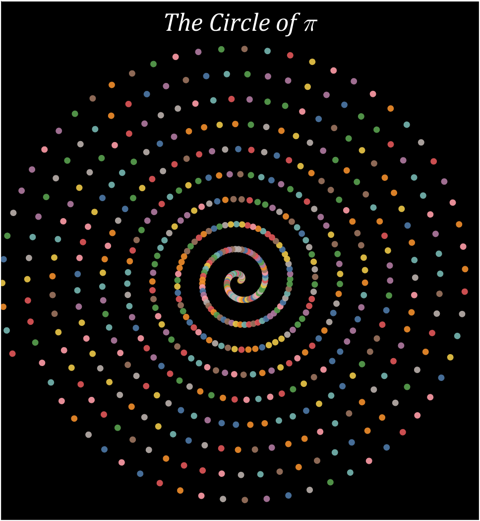
12 spiral chart
Pi=getPi(600);
CM=[78,121,167;242,142,43;225,87,89;118,183,178;89,161,79;
237,201,72;176,122,161;255,157,167;156,117,95;186,176,172]./255;
hold on
t=linspace(0,2*pi,100);
x=cos(t).*.8;
y=sin(t).*.8;
for i=1:600
X=i.*cos(i./10)./10;
Y=i.*sin(i./10)./10;
fill(X+x,Y+y,CM(Pi(i)+1,:),'EdgeColor','none','FaceAlpha',.9)
end
text(0,65,'The Circle of \pi','Color',[1,1,1],'FontName','Cambria',...
'HorizontalAlignment','center','FontSize',25,'FontAngle','italic')
set(gcf,'Position',[200,100,820,820]);
ax=gca;
ax.XLim=[-60,60];
ax.YLim=[-60,70];
ax.XTick=[];
ax.YTick=[];
ax.Color=[0,0,0];
ax.DataAspectRatio=[1,1,1];
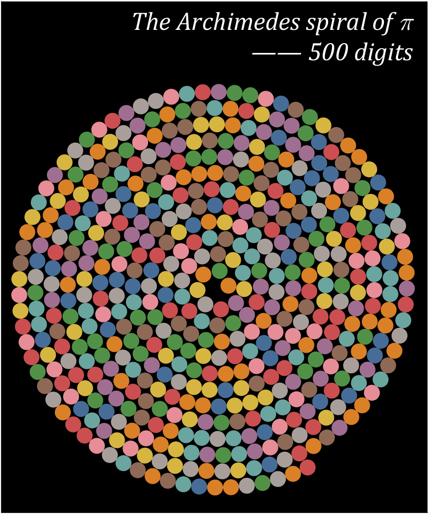
13 Archimedean spiral diagram
a=1;b=.227;
Pi=getPi(500);
CM=[78,121,167;242,142,43;225,87,89;118,183,178;89,161,79;
237,201,72;176,122,161;255,157,167;156,117,95;186,176,172]./255;
hold on
T=0;R=1;
t=linspace(0,2*pi,100);
x=cos(t).*.7;
y=sin(t).*.7;
for i=1:500
X=R.*cos(T);Y=R.*sin(T);
fill(X+x,Y+y,CM(Pi(i)+1,:),'EdgeColor','none','FaceAlpha',.9)
T=T+1./R.*1.4;
R=a+b*T;
end
text(17.25,22,{'The Archimedes spiral of \pi';'—— 500 digits'},...
'Color',[1,1,1],'FontName','Cambria',...
'HorizontalAlignment','right','FontSize',25,'FontAngle','italic')
set(gcf,'Position',[200,100,820,820]);
ax=gca;
ax.XLim=[-19,18.5];
ax.YLim=[-20,25];
ax.XTick=[];
ax.YTick=[];
ax.Color=[0,0,0];
ax.DataAspectRatio=[1,1,1];
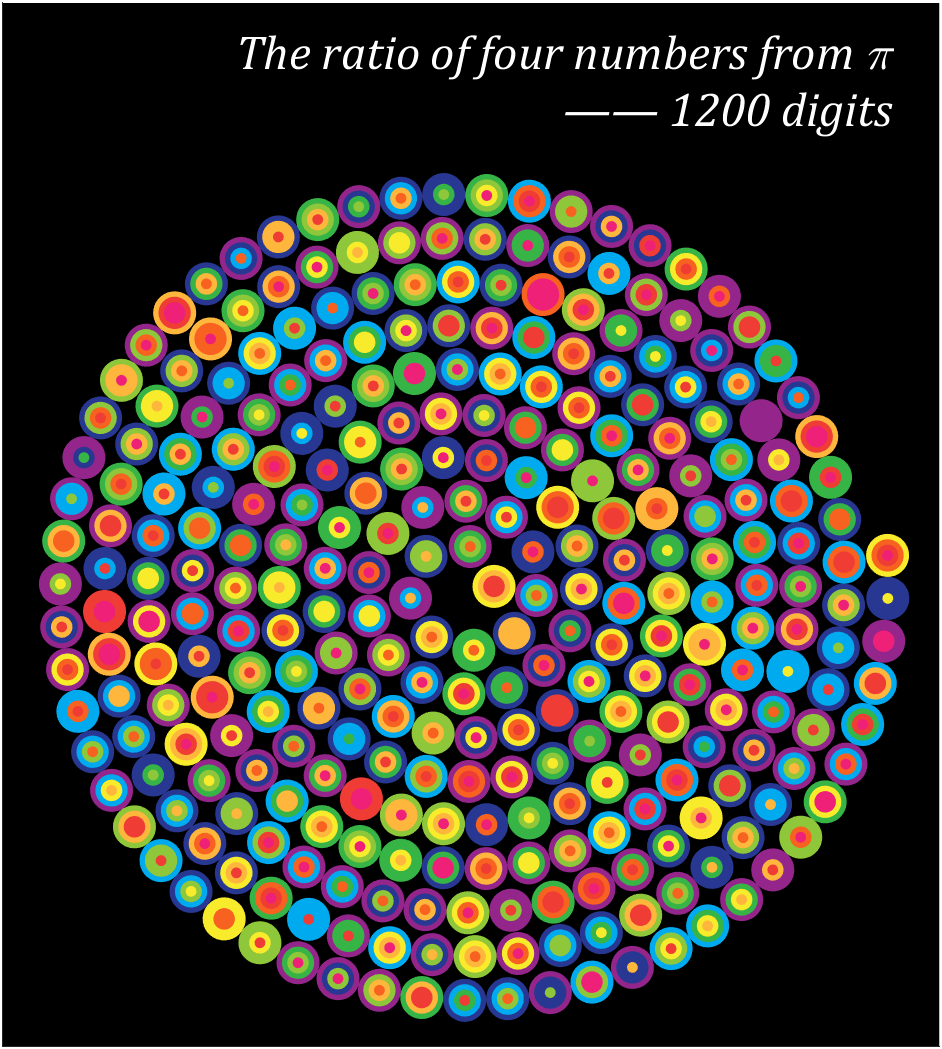
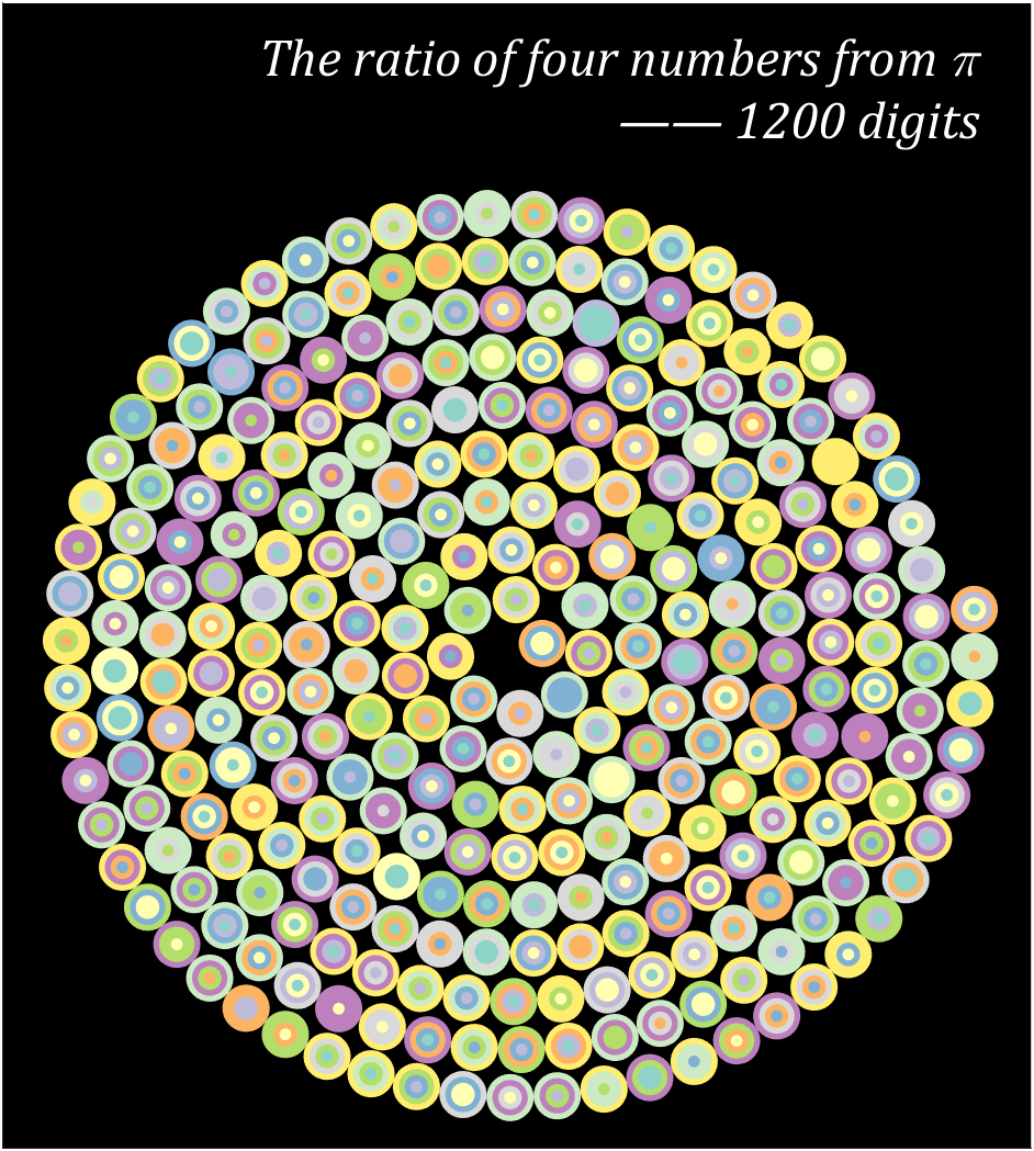
14 proportional Archimedean spiral diagram
Pi=[3,getPi(1199)];
CM=[239,32,120;239,60,52;247,98,32;255,182,60;247,235,44;
142,199,57;55,180,70;0,170,239;40,56,146;147,37,139]./255;
hold on
T=0;R=1;
t=linspace(0,2*pi,100);
x=cos(t).*.7;
y=sin(t).*.7;
for i=1:4:length(Pi)
X=R.*cos(T);Y=R.*sin(T);
tNum=Pi(i:i+3);
numNum=find([diff(sort(tNum)),1]);
numNum=[numNum(1),diff(numNum)];
cumNum=cumsum(numNum);
uniNum=unique(tNum);
for j=length(cumNum):-1:1
fill(x./4.*cumNum(j)+X,y./4.*cumNum(j)+Y,CM(uniNum(j)+1,:),'EdgeColor','none')
end
T=T+1./R.*1.4;
R=a+b*T;
end
text(14,16.5,{'The ratio of four numbers from \pi';'—— 1200 digits'},...
'Color',[1,1,1],'FontName','Cambria',...
'HorizontalAlignment','right','FontSize',23,'FontAngle','italic')
set(gcf,'Position',[200,100,820,820]);
ax=gca;
ax.XLim=[-15,15.5];
ax.YLim=[-15,19];
ax.XTick=[];
ax.YTick=[];
ax.Color=[0,0,0];
ax.DataAspectRatio=[1,1,1];
15 graph
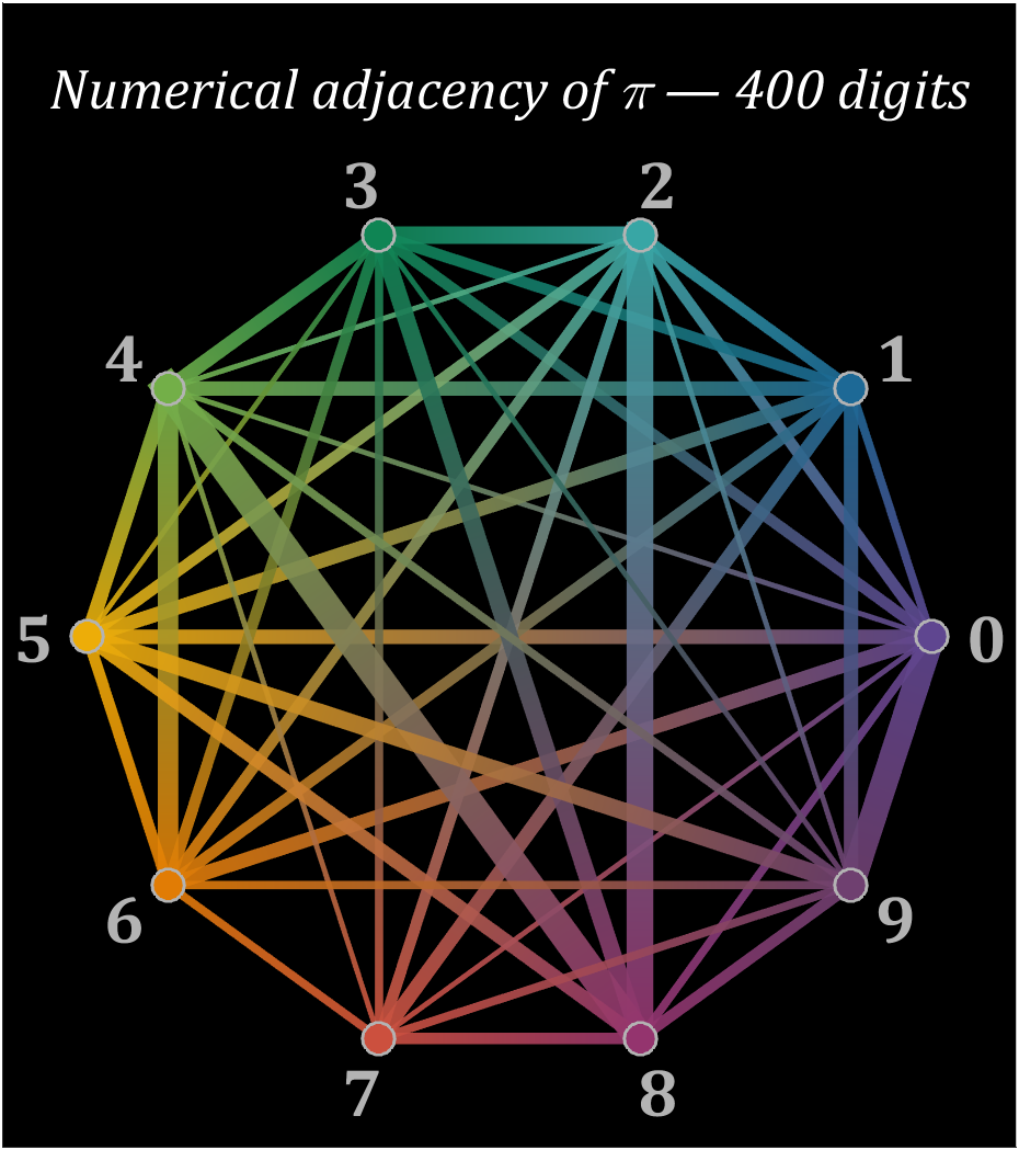
corrMat=zeros(10,10);
Pi=getPi(401);
for i=1:400
corrMat(Pi(i)+1,Pi(i+1)+1)=corrMat(Pi(i)+1,Pi(i+1)+1)+1;
end
colorList=[0.3725 0.2745 0.5647
0.1137 0.4118 0.5882
0.2196 0.6510 0.6471
0.0588 0.5216 0.3294
0.4510 0.6863 0.2824
0.9294 0.6784 0.0314
0.8824 0.4863 0.0196
0.8000 0.3137 0.2431
0.5804 0.2039 0.4314
0.4353 0.2510 0.4392];
t=linspace(0,2*pi,11);t=t(1:10)';
posXY=[cos(t),sin(t)];
maxWidth=max(corrMat(corrMat>0));
minWidth=min(corrMat(corrMat>0));
ttList=linspace(0,1,3)';
hold on
for i=1:size(corrMat,1)
for j=i+1:size(corrMat,2)
if corrMat(i,j)>0
tW=(corrMat(i,j)-minWidth)./(maxWidth-minWidth);
colorData=(1-ttList).*colorList(i,:)+ttList.*colorList(j,:);
CData(:,:,1)=colorData(:,1);
CData(:,:,2)=colorData(:,2);
CData(:,:,3)=colorData(:,3);
fill(linspace(posXY(i,1),posXY(j,1),3),...
linspace(posXY(i,2),posXY(j,2),3),[0,0,0],'LineWidth',tW.*12+1,...
'CData',CData,'EdgeColor','interp','EdgeAlpha',.7,'FaceAlpha',.7)
end
end
scatter(posXY(i,1),posXY(i,2),200,'filled','LineWidth',1.2,...
'MarkerFaceColor',colorList(i,:),'MarkerEdgeColor',[.7,.7,.7]);
text(posXY(i,1).*1.13,posXY(i,2).*1.13,num2str(i-1),'Color',[1,1,1].*.7,...
'FontSize',30,'FontWeight','bold','FontName','Cambria','HorizontalAlignment','center')
end
text(0,1.3,'Numerical adjacency of \pi — 400 digits','Color',[1,1,1],'FontName','Cambria',...
'HorizontalAlignment','center','FontSize',25,'FontAngle','italic')
set(gcf,'Position',[200,100,820,820]);
ax=gca;
ax.XLim=[-1.2,1.2];
ax.YLim=[-1.21,1.5];
ax.XTick=[];
ax.YTick=[];
ax.Color=[0,0,0];
ax.DataAspectRatio=[1,1,1];
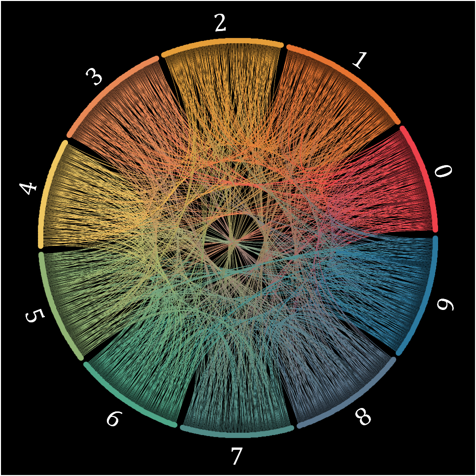
16 circos chart
Need to use this tool:
Class=getPi(1001)+1;
Data=diag(ones(1,1000),-1);
className={'0','1','2','3','4','5','6','7','8','9'};
colorOrder=[239,65,75;230,115,48;229,158,57;232,136,85;239,199,97;
144,180,116;78,166,136;81,140,136;90,118,142;43,121,159]./255;
CC=circosChart(Data,Class,'ClassName',className,'ColorOrder',colorOrder);
CC=CC.draw();
ax=gca;
ax.Color=[0,0,0];
CC.setClassLabel('Color',[1,1,1],'FontSize',25,'FontName','Cambria')
CC.setLine('LineWidth',.7)
YOU CAN GET ALL CODE HERE:

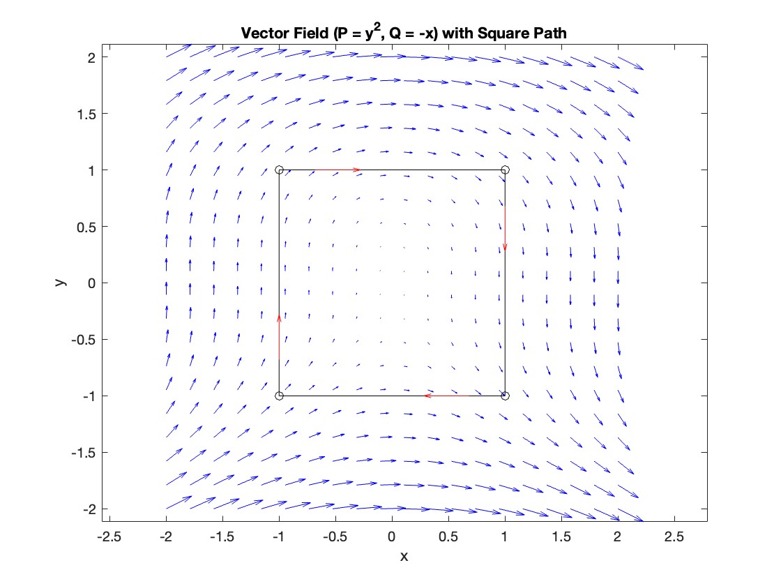
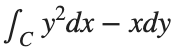 , where C is the boundary of the square
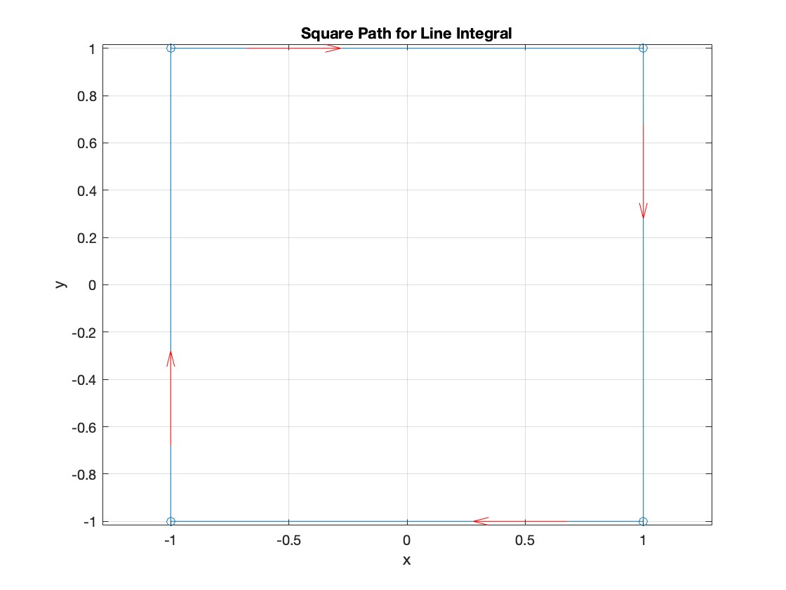
 over the sphere
  are symmetric, you can exploit these symmetries to simplify the calculation.