Results for
Have you ever learned that something you were doing manually in MATLAB was already possible using a built-in feature? Have you ever written a function only to later realize (or be told) that a built-in function already did what you needed?
Two such moments come to mind for me.
1. Did you realize that you can set conditional breakpoints? Neither did I, until someone showed me that feature. To do that, open or create a file in the editor, right click on a line number for any line that contains code, and select Set Conditional Breakpoint... This will bring up a dialog wherein you can type any logical condition for which execution should be paused. Before I learned about this, I would manually insert if-statements during debugging. Then, after fixing each bug, I would have to delete those statements. This built-in feature is so much better.
2. Have you ever needed to plot horizontal or vertical lines in a plot? For the longest time, I would manually code such lines. Then, I learned about xline() and yline(). Not only is less code required, these lines automatically span the entire axes while zooming, panning, or adjusting axis limits!
Share your own Aha! moments below. This will help everyone learn about MATLAB functionality that may not be obvious or front and center.
(Note: While File Exchange contains many great contributions, the intent of this thread is to focus on built-in MATLAB functionality.)
The carot symbol on my keyboard (ˆ shift+6) doesn't work on matlab. Matlab doesn't recognize it so I can't write any equation with power symbol. I tried every possible solution on the web and it doesn't work. even in the character viewer I don't have any result when I search ''caret".
Exciting news for students! 🚀Simulink Student Challenge 2023 is live! Unleash your engineering skills and compete for exciting rewards. Submission deadline is December 12th, 2023!

Hello all,
I've been trying to shift my workflow more towards simbiology, it has a lot of very interesting features and it makes sense to try and do everything in one place if it works well..! Part of my hesitancy into this was some bad experiences handling units in the past, though this was almost certainly all out of my own ignorance, relatedly:
Getting onto my question.
In this model I have a species traveling around the body via blow flow, think a basic PBPK model. My species are picomolarities, if everything is already in concentrations, why is it necessary to initially divide by the compartment volume? i.e. 1/Pancreas below.

If my model dealt in molar quantities this would make a lot of sense, the division would represent the transition to concentrations. This, however, now necessitates my parameters be in units of liter/minute, which is actually correct, but I'd like clarification on why it's correct, ha!
Perhaps this is more of a modelling question than a simbiology question, but if there are answers I'd love to hear them. Thanks!
Over the weekend I came across a pi approximation using durations of years and weeks (image below, Wolfram, eq. 89), accurate to 6 digits using the average Gregorian year (365.2425 days).
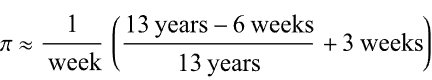
Here it is in MATLAB. I divided by 1 week at the end rather than multiplying by its reciprocal because you can’t divide a numeric by a duration in MATLAB (1/week).
weeks = @(n)n*days(7);
piApprox = ((years(13)-weeks(6))/years(13) + weeks(3)) / weeks(1)
% piApprox = 3.141593493469302
Here’s a breakdown
- The first argument becomes 12.885 yrs / 13 yrs or 0.99115
- Add three weeks: 0.99115 + 3 weeks = 21.991 days
- The reduced fraction becomes 21.991 days / 7 days
Now it looks a lot closer to the more familiar approximation for pi 22/7 but with greater precision!
Need help about FPGA Based VSC HVDC Real Time Simulation Model.
This person used computer version to build a keyboard input, and used standard flag semaphore for the positions.
Flag semaphore is used mostly by sailors to be able to communicate optically over a distance; it does not need anything more than make-shift flags (but binoculars or telescopes can help.) Trained users can go faster than you might guess.
Chen, Rena, and I are at a community management event. It's great to be with others talking about relationships, trust, and co-creation.
A research team found a way to trick a number of AI systems by injecting carefully placed nonsense -- for example being able able to beat DeepMind's Go game.
This video discusses the "Cody" bridge, which is a pedestrian bridge over a canal that has been designed to move up and out of the way when ships need to travel through. The mathematics of the bridge movement are discussed and diagrammed. It is unique and educational.
Recently developed: a "microscope" based on touch and stereo vision.
Using touch removes the possibility of optical confusion -- for example, black on touch is only due to shape, not due to the possibility that the object has a black patch.
Sorry, you might need a Facebook account to watch the video.
I'm curious how the community uses the hold command when creating charts and graphics in MATLAB. In short, hold on sets up the axes to add new objects to the axes while hold off sets up the axes to reset when new objects are added.
When you use hold on do you always follow up with hold off? What's your reasoning on this decision?
Can't wait to discuss this here! I'd love to hear from newbies and experts alike!
Calling all students! New to MATLAB or need helpful resources? Check out our MATLAB GitHub for Students repository! Find MATLAB examples, videos, cheat sheets, and more!

Visit the repository here: MATLAB GitHub for Students
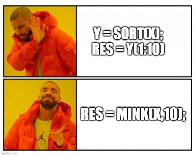
Imagine x is a large vector and you want the smallest 10 elements. How might you do it?
The way we've solved ODEs in MATLAB has been relatively unchanged at the user-level for decades. Indeed, I consider ode45 to be as iconic as backslash! There have been a few new solvers in recent years -- ode78 and ode89 for example -- and various things have gotten much faster but if you learned how to solve ODEs in MATLAB in 1997 then your knowledge is still applicable today.
In R2023b, there's a completely new framework for solving ODEs and I love it! You might argue that I'm contractually obliged to love it since I'm a MathWorker but I can assure you this is the real thing!
I wrote it up in a tutorial style on The MATLAB Blog https://blogs.mathworks.com/matlab/2023/10/03/the-new-solution-framework-for-ordinary-differential-equations-odes-in-matlab-r2023b/
The new interface makes a lot of things a much easier to do. Its also setting us up for a future where we'll be able to do some very cool algorithmic stuff behind the scenes.
Let me know what you think of the new functionality and what you think MathWorks should be doing next in the area of ODEs.
Hi All,
I'm attempting to put a set of simbiology global sensitivity analysis plots into my thesis and I'm running into some issues with the GSA plots. Firstly, the figures are very large, it would be quite beneficial to grab a set of the plots and arrange them myself, is there any documentation on how to mess around with the '1x1 Sobol' produced by sbiosobol? Or just GSA plots in general.
The second problem is that the results appear to be relative to the most sensitive parameter in that run. Is it recommended to have a resonably sensitive 'baseline' parameter in each run? I find it difficult to compare plots when a not so sensitive parameter is being recorded as near '1' for the whole run because it's being stacked against a set of very insensitive parameters. I.e. if i have multiple sets of GSAs due to a large model, how can I easily compare results? If I could do some single run through with every parameter that would be the ideal, I imagine, but then the default plot would be half a mile off the bottom of my screen, haha! Perhaps there is a solution to the first question that might help there?
Thank you for your help,
Dan
Hi all,
I've translated a model from another piece of software (monolix) into simbio programmatically to make use of your very easy global sensitivity analysis system.
It looks a little something like this, for a 'single' line example:
r1 = addreaction(model,'InsI -> InsP');
r1.ReactionRate = 'InsI*kip/vi'; %- is + panc
k1 = addkineticlaw(r1, 'Unknown');
Multiplied about 20 fold, as you can see I have included my volumes within the reaction rates myself (vi). The model functions perfectly and I have corrected the outputs at the end:
[time, x, names] = sbiosimulate(model,csObj,dObj1);
x(:,1) = x(:,1)/vi;
So that they are in concentration, as needed. However, when it comes to sensitivity analysis because I have corrected them post-model it is technically incorrect, it is analysing the absolute quantities. This is quite noticible in the sensitivity to the volumes.
Is there an easy fix to this, I've had to fight dimensionality with units in the past using simbio and I'd be great if there was some way of dividing a compartment output by a volume, for example. It is a functionality that exists in monolix, so I was hopeful it might here!
Thank you for your time.
EDIT:
I think I've worked it out, I had to refactor my model to operate in concentrations, just refitting it now. Now I should just be able to use unitless compartments.
I am trying to make a simulink model to use a MPC to reduce power consumption of HVAC system in an electric vehicle during cool down from ambient temperature to a set point temperature. Any help regarding this would be appreciated
Kindly help me correct this code to function properly. I am just learning MATLAB. i cannot get the output in abc frame. This is the code:
%----------- Define input and state parameters-----------------------------
clc
v_dc = 350; % DC input voltage in V
m = 0.841; % modulation index
C = 4000e-6; % DC buss capacitance in uf
L_1 = 2.5e-3; % Inverter side inductance in mH
L_2 = 2.5e-3; % Load side inductance in mH
L = 0; % load inductance
C_f = 10e-6; % filter capacitance in uf
R_f = 0.7; % damping resistance in ohms
R_L = 20; % load resistance in ohms
f_s = 10e3; % switching frequency
f = 60; % System frequency
R_s = 0.01; % Capacitance of the DC circuit
I_d = 8.594; % steady state current
w = 2*pi*f; % System angular Frequency
% Define initial steady state values
v_c = 349.4; i_d = 8.594; i_q = -0.213; v_df = 285; v_qf = -120; i_Ld = 8.594; i_Lq = 0.85;
%------------------S V P W M Generator-------------------------------------
% Define reference vector Uref
U_mag = m*v_dc/2; % Magnitude of Uref
% Define switching vectors
U1 = [v_dc/2;0]; % Vector Q1
U2 = [v_dc/4;sqrt(3)*v_dc/4]; % Vector Q2
U3 = [-v_dc/4;sqrt(3)*v_dc/4]; % Vector Q3
U4 = [-v_dc/2;0]; % Vector Q4
U5 = [-v_dc/4;-sqrt(3)*v_dc/4]; % Vector Q5
U6 = [v_dc/4;-sqrt(3)*v_dc/4]; % Vector Q6
% Define sector angles
theta1 = pi/6;
theta2 = pi/2;
theta3 = 5*pi/6;
theta4 = 7*pi/6;
theta5 = 3*pi/2;
theta6 = 11*pi/6;
% Define duty cycles for each switch using a for loop
for t=0:1/f_s:1/f % Time variable from 0 to one cycle of system frequency with steps of switching frequency
U_phase = w*t; % Phase of Uref (t is time variable)
U_alpha = U_mag*cos(U_phase); % Alpha component of Uref
U_beta = U_mag*sin(U_phase); % Beta component of Uref
if (0 <= U_phase) && (U_phase < theta1) % Sector 1
T1 = (sqrt(3)*U_beta + U_alpha)/(2*v_dc);
T2 = (-sqrt(3)*U_beta + U_alpha)/(2*v_dc);
T0 = 1 - T1 - T2;
d_a(round(t)+1) = T1 + T0/2;
d_b(round(t)+1) = T2 + T0/2;
d_c(round(t)+1) = T0/2;
elseif (theta1 <= U_phase) && (U_phase < theta2) % Sector 2
T3 = (sqrt(3)*U_beta - U_alpha)/(2*v_dc);
T2 = (sqrt(3)*U_beta + U_alpha)/(2*v_dc);
T0 = 1 - T3 - T2;
d_a(round(t)+1) = T0/2;
d_b(round(t)+1) = T2 + T0/2;
d_c(round(t)+1) = T3 + T0/2;
elseif (theta2 <= U_phase) && (U_phase < theta3) % Sector 3
T3 = (sqrt(3)*U_beta - U_alpha)/(2*v_dc);
T4 = (-sqrt(3)*U_beta - U_alpha)/(2*v_dc);
T0 = 1 - T3 - T4;
d_a(round(t)+1) = T0/2;
d_b(round(t)+1) = T0/2;
d_c(round(t)+1) = T3 + T0/2;
elseif (theta3 <= U_phase) && (U_phase < theta4) % Sector 4
T5 = (-sqrt(3)*U_beta + U_alpha)/(2*v_dc);
T4 = (-sqrt(3)*U_beta - U_alpha)/(2*v_dc);
T0 = 1 - T5 - T4;
d_a(round(t)+1) = T5 + T0/2;
d_b(round(t)+1) = T0/2;
d_c(round(t)+1) = T4 + T0/2;
elseif (theta4 <= U_phase) && (U_phase < theta5) % Sector 5
T5 = (-sqrt(3)*U_beta + U_alpha)/(2*v_dc);
T6 = (sqrt(3)*U_beta + U_alpha)/(2*v_dc);
T0 = 1 - T5 - T6;
d_a(round(t)+1) = T5 + T0/2;
d_b(round(t)+1) = T6 + T0/2;
d_c(round(t)+1) = T0/2;
elseif (theta5 <= U_phase) && (U_phase < theta6) % Sector 6
T1 = (sqrt(3)*U_beta + U_alpha)/(2*v_dc);
T6 = (sqrt(3)*U_beta - U_alpha)/(2*v_dc);
T0 = 1 - T1 - T6;
d_a(round(t)+1) = T1 + T0/2;
d_b(round(t)+1) = T0/2;
d_c(round(t)+1) = T6 + T0/2;
end
end
%-------------------------Define system matrices---------------------------
% Create Three-phase SVPWM VSI Inverter
% System matrix Nx-by-Nx matrix
A = [-1/(C*R_s),-sqrt(3)*m/(2*C),0,0,0,0,0;
sqrt(3)*m/(3*L_1),-R_f/(3*L_1),w,-1/(2*L_1),-sqrt(3)/(6*L_1),-R_f/(3*L_1),0;
0,-w,-R_f/(3*L_1),-sqrt(3)/(6*L_1),-1/(2*L_1),0,R_f/(3*L_1);
0,1/(2*C_f),-sqrt(3)/(6*C_f),0,w,-1/(2*C_f),sqrt(3)/(6*C_f);
0,sqrt(3)/(6*C_f),1/(2*C_f),-w,0,-sqrt(3)/(6*C_f),-1/(2*C_f);
0,R_f/(3*(L_2+L)),0,1/(2*(L_2+L)),sqrt(3)/(6*(L_2+L)),((-3*R_L-R_f)/(3*(L_2+L))),w;
0, 0, R_f/(3*(L_2+L)), -sqrt(3)/(6*(L_2+L)), 1/(2*(L_2+L)), -w, ((-3*R_L-R_f)/(3*(L_2+L)))];
% Define input matrix
B = [1/(C*R_s),-sqrt(3)*i_d/(2*C);d_a*v_dc,(sqrt(3)*v_c)/L_1;d_b*v_dc,0;d_c*v_dc,0;0,0;0,0;0,0]; % Nx-by-Nu input matrix
% Define output matrix
C = [0 1 0 0 0 0 0; % Ny-by-Nx matrix
0 0 1 0 0 0 0;
0 0 0 1 0 0 0;
0 0 0 0 1 0 0;
0 0 0 0 0 1 0;
0 0 0 0 0 0 1];
% Feedthrough matrix
D = zeros(6, 2); % Ny-by-Nu matrix
% create state-space model object
sys = ss(A,B,C,D);
% Define initial conditions and input
x0 = [v_c; i_d; i_q; v_df; v_qf; i_Ld; i_Lq]; % Initial state vector
t = 0:1e-6:0.5; % Time vector for simulation
u = repmat([v_dc;m],1,length(t)); % repeat u for each time step
% Simulate the system
[y, ~, x] = lsim(sys, u, t, x0);
% Extract the states
v_c_sim = x(:, 1);
i_d_sim = x(:, 2);
i_q_sim = x(:, 3);
v_df_sim = x(:, 4);
v_qf_sim = x(:, 5);
i_Ld_sim = x(:, 6);
i_Lq_sim = x(:, 7);
% Extract the outputs
v_abc_sim = y(:, 1:3);
i_abc_sim = y(:, 4:6);
v_dq_sim = y(:, 4:5);
i_dq_sim = y(:, 2:3);
% Plot the variables
figure;
subplot(4, 2, 1);
plot(t, v_c_sim);
xlabel('Time');
ylabel('v_c');
title('Capacitor Voltage');
subplot(4, 2, 2);
plot(t, i_d_sim);
xlabel('Time');
ylabel('i_d');
title('d-Axis Current');
subplot(4, 2, 3);
plot(t, i_q_sim);
xlabel('Time');
ylabel('i_q');
title('q-Axis Current');
subplot(4, 2, 4);
plot(t, v_df_sim);
xlabel('Time');
ylabel('v_df');
title('d-Component Filter Voltage');
subplot(4, 2, 5);
plot(t, v_qf_sim);
xlabel('Time');
ylabel('v_qf');
title('q-Component Filter Voltage');
subplot(4, 2, 6);
plot(t, i_Ld_sim);
xlabel('Time');
ylabel('i_Ld');
title('d-Axis Load Current');
subplot(4, 2, 7);
plot(t, i_Lq_sim);
xlabel('Time');
ylabel('i_Lq');
title('q-Axis Load Current');
% Perform coordinate transformation from dq frame to abc frame for currents
i_a_sim = cos(w*t)*i_d_sim - sin(w*t)*i_q_sim;
i_b_sim = cos(w*t - 2*pi/3)*i_d_sim - sin(w*t - 2*pi/3)*i_q_sim;
i_c_sim = cos(w*t + 2*pi/3)*i_d_sim - sin(w*t + 2*pi/3)*i_q_sim;
% Perform coordinate transformation from dq frame to abc frame for voltages
v_a_sim = cos(w*t)*v_df_sim - sin(w*t)*v_qf_sim;
v_b_sim = cos(w*t - 2*pi/3)*v_df_sim - sin(w*t - 2*pi/3)*v_qf_sim;
v_c_sim = cos(w*t + 2*pi/3)*v_df_sim - sin(w*t + 2*pi/3)*v_qf_sim;
Many thanks
I am trying to simulate model of blood lymphocyte count from a paper using Simbiology. The rate of in or out following circadian rythym is kp(t)=km + kb cos [(t-tpeak)*2pi/24] Where and how do I write the expression ? I dont think I can write in repeated assignment ?