R =
Results for
I saw an interesting problem on a reddit math forum today. The question was to find a number (x) as close as possible to r=3.6, but the requirement is that both x and 1/x be representable in a finite number of decimal places.
The problem of course is that 3.6 = 18/5. And the problem with 18/5 has an inverse 5/18, which will not have a finite representation in decimal form.
In order for a number and its inverse to both be representable in a finite number of decimal places (using base 10) we must have it be of the form 2^p*5^q, where p and q are integer, but may be either positive or negative. If that is not clear to you intuitively, suppose we have a form
2^p*5^-q
where p and q are both positive. All you need do is multiply that number by 10^q. All this does is shift the decimal point since you are just myltiplying by powers of 10. But now the result is
2^(p+q)
and that is clearly an integer, so the original number could be represented using a finite number of digits as a decimal. The same general idea would apply if p was negative, or if both of them were negative exponents.
Now, to return to the problem at hand... We can obviously adjust the number r to be 20/5 = 4, or 16/5 = 3.2. In both cases, since the fraction is now of the desired form, we are happy. But neither of them is really close to 3.6. My goal will be to find a better approximation, but hopefully, I can avoid a horrendous amount of trial and error. It would seem the trick might be to take logs, to get us closer to a solution. That is, suppose I take logs, to the base 2?
log2(3.6)
I used log2 here because that makes the problem a little simpler, since log2(2^p)=p. Therefore we want to find a pair of integers (p,q) such that
log2(3.6) + delta = p + log2(5)*q
where delta is as close to zero as possible. Thus delta is the error in our approximation to 3.6. And since we are working in logs, delta can be viewed as a proportional error term. Again, p and q may be any integers, either positive or negative. The two cases we have seen already have (p,q) = (2,0), and (4,-1).
Do you see the general idea? The line we have is of the form
log2(3.6) = p + log2(5)*q
it represents a line in the (p,q) plane, and we want to find a point on the integer lattice (p,q) where the line passes as closely as possible.
[Xl,Yl] = meshgrid([-10:10]);
plot(Xl,Yl,'k.')
hold on
fimplicit(@(p,q) -log2(3.6) + p + log2(5)*q,[-10,10,-10,10],'g-')
plot([2 4],[0,-1],'ro')
hold off
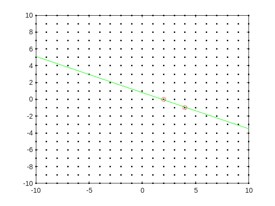
Now, some might think in terms of orthogonal distance to the line, but really, we want the vertical distance to be minimized. Again, minimize abs(delta) in the equation:
log2(3.6) + delta = p + log2(5)*q
where p and q are integer.
Can we do that using MATLAB? The skill about about mathematics often lies in formulating a word problem, and then turning the word problem into a problem of mathematics that we know how to solve. We are almost there now. I next want to formulate this into a problem that intlinprog can solve. The problem at first is intlinprog cannot handle absolute value constraints. And the trick there is to employ slack variables, a terribly useful tool to emply on this class of problem.
Rewrite delta as:
delta = Dpos - Dneg
where Dpos and Dneg are real variables, but both are constrained to be positive.
prob = optimproblem;
p = optimvar('p',lower = -50,upper = 50,type = 'integer');
q = optimvar('q',lower = -50,upper = 50,type = 'integer');
Dpos = optimvar('Dpos',lower = 0);
Dneg = optimvar('Dneg',lower = 0);
Our goal for the ILP solver will be to minimize Dpos + Dneg now. But since they must both be positive, it solves the min absolute value objective. One of them will always be zero.
r = 3.6;
prob.Constraints = log2(r) + Dpos - Dneg == p + log2(5)*q;
prob.Objective = Dpos + Dneg;
The solve is now a simple one. I'll tell it to use intlinprog, even though it would probably figure that out by itself. (Note: if I do not tell solve which solver to use, it does use intlinprog. But it also finds the correct solution when I told it to use GA offline.)
solve(prob,solver = 'intlinprog')
The solution it finds within the bounds of +/- 50 for both p and q seems pretty good. Note that Dpos and Dneg are pretty close to zero.
2^39*5^-16
and while 3.6028979... seems like nothing special, in fact, it is of the form we want.
R = sym(2)^39*sym(5)^-16
vpa(R,100)
vpa(1/R,100)
both of those numbers are exact. If I wanted to find a better approximation to 3.6, all I need do is extend the bounds on p and q. And we can use the same solution approch for any floating point number.
Registration is now open for MathWorks annual virtual event MATLAB EXPO 2025 on November 12 – 13, 2025!
Register now and start building your customized agenda today!
Explore. Experience. Engage.
Join MATLAB EXPO to connect with MathWorks and industry experts to learn about the latest trends and advancements in engineering and science. You will discover new features and capabilities for MATLAB and Simulink that you can immediately apply to your work.

For some time now, this has been bugging me - so I thought to gather some more feedback/information/opinions on this.
What would you classify Recursion? As a loop or as a vectorized section of code?
For context, this query occured to me while creating Cody problems involving strict (so to speak) vectorization - (Everyone is more than welcome to check my recent Cody questions).
To make problems interesting and/or difficult, I (and other posters) ban functions and functionalities - such as for loops, while loops, if-else statements, arrayfun() and the rest of the fun() family functions. However, some of the solutions including the reference solution I came up with for my latest problem, contained recursion.
I am rather divided on how to categorize it. What do you think?
Since R2024b, a Levenberg–Marquardt solver (TrainingOptionsLM) was introduced. The built‑in function trainnet now accepts training options via the trainingOptions function (https://www.mathworks.com/help/deeplearning/ref/trainingoptions.html#bu59f0q-2) and supports the LM algorithm. I have been curious how to use it in deep learning, and the official documentation has not provided a concrete usage example so far. Below I give a simple example to illustrate how to use this LM algorithm to optimize a small number of learnable parameters.
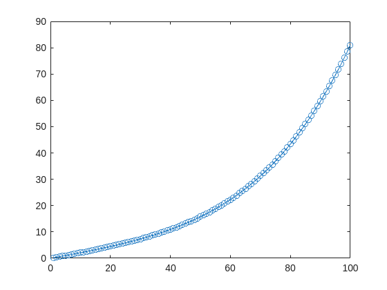
For example, consider the nonlinear function:
y_hat = @(a,t) a(1)*(t/100) + a(2)*(t/100).^2 + a(3)*(t/100).^3 + a(4)*(t/100).^4;
It represents a curve. Given 100 matching points (t → y_hat), we want to use least squares to estimate the four parameters a1–a4.
t = (1:100)';
y_hat = @(a,t)a(1)*(t/100) + a(2)*(t/100).^2 + a(3)*(t/100).^3 + a(4)*(t/100).^4;
x_true = [ 20 ; 10 ; 1 ; 50 ];
y_true = y_hat(x_true,t);
plot(t,y_true,'o-')
- Using the traditional lsqcurvefit-wrapped "Levenberg–Marquardt" algorithm:
x_guess = [ 5 ; 2 ; 0.2 ; -10 ];
options = optimoptions("lsqcurvefit",Algorithm="levenberg-marquardt",MaxFunctionEvaluations=800);
[x,resnorm,residual,exitflag] = lsqcurvefit(y_hat,x_guess,t,y_true,-50*ones(4,1),60*ones(4,1),options);
x,resnorm,exitflag
- Using the deep-learning-wrapped "Levenberg–Marquardt" algorithm:
options = trainingOptions("lm", ...
InitialDampingFactor=0.002, ...
MaxDampingFactor=1e9, ...
DampingIncreaseFactor=12, ...
DampingDecreaseFactor=0.2,...
GradientTolerance=1e-6, ...
StepTolerance=1e-6,...
Plots="training-progress");
numFeatures = 1;
layers = [featureInputLayer(numFeatures,'Name','input')
fitCurveLayer(Name='fitCurve')];
net = dlnetwork(layers);
XData = dlarray(t);
YData = dlarray(y_true);
netTrained = trainnet(XData,YData,net,"mse",options);
netTrained.Layers(2)
classdef fitCurveLayer < nnet.layer.Layer ...
& nnet.layer.Acceleratable
% Example custom SReLU layer.
properties (Learnable)
% Layer learnable parameters
a1
a2
a3
a4
end
methods
function layer = fitCurveLayer(args)
arguments
args.Name = "lm_fit";
end
% Set layer name.
layer.Name = args.Name;
% Set layer description.
layer.Description = "fit curve layer";
end
function layer = initialize(layer,~)
% layer = initialize(layer,layout) initializes the layer
% learnable parameters using the specified input layout.
if isempty(layer.a1)
layer.a1 = rand();
end
if isempty(layer.a2)
layer.a2 = rand();
end
if isempty(layer.a3)
layer.a3 = rand();
end
if isempty(layer.a4)
layer.a4 = rand();
end
end
function Y = predict(layer, X)
% Y = predict(layer, X) forwards the input data X through the
% layer and outputs the result Y.
% Y = layer.a1.*exp(-X./layer.a2) + layer.a3.*X.*exp(-X./layer.a4);
Y = layer.a1*(X/100) + layer.a2*(X/100).^2 + layer.a3*(X/100).^3 + layer.a4*(X/100).^4;
end
end
end
The network is very simple — only the fitCurveLayer defines the learnable parameters a1–a4. I observed that the output values are very close to those from lsqcurvefit.
Function Syntax Design Conundrum
As a MATLAB enthusiast, I particularly enjoy Steve Eddins' blog and the cool things he explores. MATLAB's new argument blocks are great, but there's one frustrating limitation that Steve outlined beautifully in his blog post "Function Syntax Design Conundrum": cases where an argument should accept both enumerated values AND other data types.
Steve points out this could be done using the input parser, but I prefer having tab completions and I'm not a fan of maintaining function signature JSON files for all my functions.
Personal Context on Enumerations
To be clear: I honestly don't like enumerations in any way, shape, or form. One reason is how awkward they are. I've long suspected they're simply predefined constructor calls with a set argument, and I think that's all but confirmed here. This explains why I've had to fight the enumeration system when trying to take arguments of many types and normalize them to enumerated members, or have numeric values displayed as enumerated members without being recast to the superclass every operation.
The Discovery
While playing around extensively with metadata for another project, I realized (and I'm entirely unsure why it took so long) that the properties of a metaclass object are just, in many cases, the attributes of the classdef. In this realization, I found a solution to Steve's and my problem.
To be clear: I'm not in love with this solution. I would much prefer a better approach for allowing variable sets of membership validation for arguments. But as it stands, we don't have that, so here's an interesting, if incredibly hacky, solution.
If you call struct() on a metaclass object to view its hidden properties, you'll notice that in addition to the public "Enumeration" property, there's a hidden "Enumerable" property. They're both logicals, which implies they're likely functionally distinct. I was curious about that distinction and hoped to find some functionality by intentionally manipulating these values - and I did, solving the exact problem Steve mentions.
The Problem Statement
We have a function with an argument that should allow "dual" input types: enumerated values (Steve's example uses days of the week, mine uses the "all" option available in various dimension-operating functions) AND integers. We want tab completion for the enumerated values while still accepting the numeric inputs.
A Solution for Tab-Completion Supported Arguments
Rather than spoil Steve's blog post, let me use my own example: implementing a none() function. The definition is simple enough tf = ~any(A, dim); but when we wrap this in another function, we lose the tab-completion that any() provides for the dim argument (which gives you "all"). There's no great way to implement this as a function author currently - at least, that's well documented.
So here's my solution:
%% Example Function Implementation
% This is a simple implementation of the DimensionArgument class for implementing dual type inputs that allow enumerated tab-completion.
function tf = none(A, dim)
arguments(Input)
A logical;
dim DimensionArgument = DimensionArgument(A, true);
end
% Simple example (notice the use of uplus to unwrap the hidden property)
tf = ~any(A, +dim);
end
I like this approach because the additional work required to implement it, once the enumeration class is initialized, is minimal. Here are examples of function calls, note that the behavior parallels that of the MATLAB native-style tab-completion:
%% Test Data
% Simple logical array for testing
A = randi([0, 1], [3, 5], "logical");
%% Example function calls
tf = none(A, "all"); % This is the tab-completion it's 1:1 with MATLABs behavior
tf = none(A, [1, 2]); % We can still use valid arguments (validated in the constructor)
tf = none(A); % Showcase of the constructors use as a default argument generator
How It Works
What makes this work is the previously mentioned Enumeration attribute. By setting Enumeration = false while still declaring an enumeration block in the classdef file, we get the suggested members as auto-complete suggestions. As I hinted at, the value of enumerations (if you don't subclass a builtin and define values with the someMember (1) syntax) are simply arguments to constructor calls.
We also get full control over the storage and handling of the class, which means we lose the implicit storage that enumerations normally provide and are responsible for doing so ourselves - but I much prefer this. We can implement internal validation logic to ensure values that aren't in the enumerated set still comply with our constraints, and store the input (whether the enumerated member or alternative type) in an internal property.
As seen in the example class below, this maintains a convenient interface for both the function caller and author the only particuarly verbose portion is the conversion methods... Which if your willing to double down on the uplus unwrapping context can be avoided. What I have personally done is overload the uplus function to return the input (or perform the identity property) this allowss for the uplus to be used universally to unwrap inputs and for those that cant, and dont have a uplus definition, the value itself is just returned:
classdef(Enumeration = false) DimensionArgument % < matlab.mixin.internal.MatrixDisplay
%DimensionArgument Enumeration class to provide auto-complete on functions needing the dimension type seen in all()
% Enumerations are just macros to make constructor calls with a known set of arguments. Declaring the 'all'
% enumeration member means this class can be set as the type for an input and the auto-completion for the given
% argument will show the enumeration members, allowing tab-completion. Declaring the Enumeration attribute of
% the class as false gives us control over the constructor and internal implementation. As such we can use it
% to validate the numeric inputs, in the event the 'all' option was not used, and return an object that will
% then work in place of valid dimension argument options.
%% Enumeration members
% These are the auto-complete options you'd like to make available for the function signature for a given
% argument.
enumeration(Description="Enumerated value for the dimension argument.")
all
end
%% Properties
% The internal property allows the constructor's input to be stored; this ensures that the value is store and
% that the output of the constructor has the class type so that the validation passes.
% (Constructors must return the an object of the class they're a constructor for)
properties(Hidden, Description="Storage of the constructor input for later use.")
Data = [];
end
%% Constructor method
% By the magic of declaring (Enumeration = false) in our class def arguments we get full control over the
% constructor implementation.
%
% The second argument in this specific instance is to enable the argument's default value to be set in the
% arguments block itself as opposed to doing so in the function body... I like this better but if you didn't
% you could just as easily keep the constructor simple.
methods
function obj = DimensionArgument(A, Adim)
%DimensionArgument Initialize the dimension argument.
arguments
% This will be the enumeration member name from auto-completed entries, or the raw user input if not
% used.
A = [];
% A flag that indicates to create the value using different logic, in this case the first non-singleton
% dimension, because this matches the behavior of functions like, all(), sum() prod(), etc.
Adim (1, 1) logical = false;
end
if(Adim)
% Allows default initialization from an input to match the aforemention function's behavior
obj.Data = firstNonscalarDim(A);
else
% As a convenience for this style of implementation we can validate the input to ensure that since we're
% suppose to be an enumeration, the input is valid
DimensionArgument.mustBeValidMember(A);
% Store the input in a hidden property since declaring ~Enumeration means we are responsible for storing
% it.
obj.Data = A;
end
end
end
%% Conversion methods
% Applies conversion to the data property so that implicit casting of functions works. Unfortunately most of
% the MathWorks defined functions use a different system than that employed by the arguments block, which
% defers to the class defined converter methods... Which is why uplus (+obj) has been defined to unwrap the
% data for ease of use.
methods
function obj = uplus(obj)
obj = obj.Data;
end
function str = char(obj)
str = char(obj.Data);
end
function str = cellstr(obj)
str = cellstr(obj.Data);
end
function str = string(obj)
str = string(obj.Data);
end
function A = double(obj)
A = double(obj.Data);
end
function A = int8(obj)
A = int8(obj.Data);
end
function A = int16(obj)
A = int16(obj.Data);
end
function A = int32(obj)
A = int32(obj.Data);
end
function A = int64(obj)
A = int64(obj.Data);
end
end
%% Validation methods
% These utility methods are for input validation
methods(Static, Access = private)
function tf = isValidMember(obj)
%isValidMember Checks that the input is a valid dimension argument.
tf = (istext(obj) && all(obj == "all", "all")) || (isnumeric(obj) && all(isint(obj) & obj > 0, "all"));
end
function mustBeValidMember(obj)
%mustBeValidMember Validates that the input is a valid dimension argument for the dim/dimVec arguments.
if(~DimensionArgument.isValidMember(obj))
exception("JB:DimensionArgument:InvalidInput", "Input must be an integer value or the term 'all'.")
end
end
end
%% Convenient data display passthrough
methods
function disp(obj, name)
arguments
obj DimensionArgument
name string {mustBeScalarOrEmpty} = [];
end
% Dispatch internal data's display implementation
display(obj.Data, char(name));
end
end
end
In the event you'd actually play with theres here are the function definitions for some of the utility functions I used in them, including my exception would be a pain so i wont, these cases wont use it any...
% Far from my definition isint() but is consistent with mustBeInteger() for real numbers but will suffice for the example
function tf = isint(A)
arguments
A {mustBeNumeric(A)};
end
tf = floor(A) == A
end
% Sort of the same but its fine
function dim = firstNonscalarDim(A)
arguments
A
end
dim = [find(size(A) > 1, 1), 0];
dim(1) = dim(1);
end
Hello MATLAB Central, this is my first article.
My name is Yann. And I love MATLAB.
I also love HTTP (i know, weird fetish)
So i started a conversation with ChatGPT about it:
gitclone('https://github.com/yanndebray/HTTP-with-MATLAB');
cd('HTTP-with-MATLAB')
http_with_MATLAB
I'm not sure that this platform is intended to clone repos from github, but i figured I'd paste this shortcut in case you want to try out my live script http_with_MATLAB.m
A lot of what i program lately relies on external web services (either for fetching data, or calling LLMs).
So I wrote a small tutorial of the 7 or so things I feel like I need to remember when making HTTP requests in MATLAB.
Let me know what you think
Did you know that function double with string vector input significantly outperforms str2double with the same input:
x = rand(1,50000);
t = string(x);
tic; str2double(t); toc
tic; I1 = str2double(t); toc
tic; I2 = double(t); toc
isequal(I1,I2)
Recently I needed to parse numbers from text. I automatically tried to use str2double. However, profiling revealed that str2double was the main bottleneck in my code. Than I realized that there is a new note (since R2024a) in the documentation of str2double:
"Calling string and then double is recommended over str2double because it provides greater flexibility and allows vectorization. For additional information, see Alternative Functionality."
Hey cody fellows :-) !
I recently created two problem groups, but as you can see I struggle to set their cover images :
What is weird given :
- I already did it successfully twice in the past for my previous groups ;
- If you take one problem specifically, Problem 60984. Mesh the icosahedron for instance, you can normally see the icon of the cover image in the top right hand corner, can't you ?
- I always manage to set cover images to my contributions (mostly in the filexchange).
I already tried several image formats, included .png 4/3 ratio, but still the cover images don't set.
Could you please help me to correctly set my cover images ?
Thank you.
Nicolas
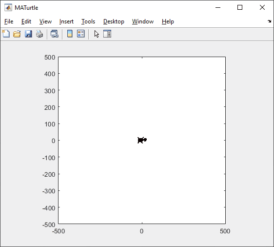
t = turtle(); % Start a turtle
t.forward(100); % Move forward by 100
t.backward(100); % Move backward by 100
t.left(90); % Turn left by 90 degrees
t.right(90); % Tur right by 90 degrees
t.goto(100, 100); % Move to (100, 100)
t.turnto(90); % Turn to 90 degrees, i.e. north
t.speed(1000); % Set turtle speed as 1000 (default: 500)
t.pen_up(); % Pen up. Turtle leaves no trace.
t.pen_down(); % Pen down. Turtle leaves a trace again.
t.color('b'); % Change line color to 'b'
t.begin_fill(FaceColor, EdgeColor, FaceAlpha); % Start filling
t.end_fill(); % End filling
t.change_icon('person.png'); % Change the icon to 'person.png'
t.clear(); % Clear the Axes
classdef turtle < handle
properties (GetAccess = public, SetAccess = private)
x = 0
y = 0
q = 0
end
properties (SetAccess = public)
speed (1, 1) double = 500
end
properties (GetAccess = private)
speed_reg = 100
n_steps = 20
ax
l
ht
im
is_pen_up = false
is_filling = false
fill_color
fill_alpha
end
methods
function obj = turtle()
figure(Name='MATurtle', NumberTitle='off')
obj.ax = axes(box="on");
hold on,
obj.ht = hgtransform();
icon = flipud(imread('turtle.png'));
obj.im = imagesc(obj.ht, icon, ...
XData=[-30, 30], YData=[-30, 30], ...
AlphaData=(255 - double(rgb2gray(icon)))/255);
obj.l = plot(obj.x, obj.y, 'k');
obj.ax.XLim = [-500, 500];
obj.ax.YLim = [-500, 500];
obj.ax.DataAspectRatio = [1, 1, 1];
obj.ax.Toolbar.Visible = 'off';
disableDefaultInteractivity(obj.ax);
end
function home(obj)
obj.x = 0;
obj.y = 0;
obj.ht.Matrix = eye(4);
end
function forward(obj, dist)
obj.step(dist);
end
function backward(obj, dist)
obj.step(-dist)
end
function step(obj, delta)
if numel(delta) == 1
delta = delta*[cosd(obj.q), sind(obj.q)];
end
if obj.is_filling
obj.fill(delta);
else
obj.move(delta);
end
end
function goto(obj, x, y)
dx = x - obj.x;
dy = y - obj.y;
obj.turnto(rad2deg(atan2(dy, dx)));
obj.step([dx, dy]);
end
function left(obj, q)
obj.turn(q);
end
function right(obj, q)
obj.turn(-q);
end
function turnto(obj, q)
obj.turn(obj.wrap_angle(q - obj.q, -180));
end
function pen_up(obj)
if obj.is_filling
warning('not available while filling')
return
end
obj.is_pen_up = true;
end
function pen_down(obj, go)
if obj.is_pen_up
if nargin == 1
obj.l(end+1) = plot(obj.x, obj.y, Color=obj.l(end).Color);
else
obj.l(end+1) = go;
end
uistack(obj.ht, 'top')
end
obj.is_pen_up = false;
end
function color(obj, line_color)
if obj.is_filling
warning('not available while filling')
return
end
obj.pen_up();
obj.pen_down(plot(obj.x, obj.y, Color=line_color));
end
function begin_fill(obj, FaceColor, EdgeColor, FaceAlpha)
arguments
obj
FaceColor = [.6, .9, .6];
EdgeColor = [0 0.4470 0.7410];
FaceAlpha = 1;
end
if obj.is_filling
warning('already filling')
return
end
obj.fill_color = FaceColor;
obj.fill_alpha = FaceAlpha;
obj.pen_up();
obj.pen_down(patch(obj.x, obj.y, [1, 1, 1], ...
EdgeColor=EdgeColor, FaceAlpha=0));
obj.is_filling = true;
end
function end_fill(obj)
if ~obj.is_filling
warning('not filling now')
return
end
obj.l(end).FaceColor = obj.fill_color;
obj.l(end).FaceAlpha = obj.fill_alpha;
obj.is_filling = false;
end
function change_icon(obj, filename)
icon = flipud(imread(filename));
obj.im.CData = icon;
obj.im.AlphaData = (255 - double(rgb2gray(icon)))/255;
end
function clear(obj)
obj.x = 0;
obj.y = 0;
delete(obj.ax.Children(2:end));
obj.l = plot(0, 0, 'k');
obj.ht.Matrix = eye(4);
end
end
methods (Access = private)
function animated_step(obj, delta, q, initFcn, updateFcn)
arguments
obj
delta
q
initFcn = @() []
updateFcn = @(~, ~) []
end
dx = delta(1)/obj.n_steps;
dy = delta(2)/obj.n_steps;
dq = q/obj.n_steps;
pause_duration = norm(delta)/obj.speed/obj.speed_reg;
initFcn();
for i = 1:obj.n_steps
updateFcn(dx, dy);
obj.ht.Matrix = makehgtform(...
translate=[obj.x + dx*i, obj.y + dy*i, 0], ...
zrotate=deg2rad(obj.q + dq*i));
pause(pause_duration)
drawnow limitrate
end
obj.x = obj.x + delta(1);
obj.y = obj.y + delta(2);
end
function obj = turn(obj, q)
obj.animated_step([0, 0], q);
obj.q = obj.wrap_angle(obj.q + q, 0);
end
function move(obj, delta)
initFcn = @() [];
updateFcn = @(dx, dy) [];
if ~obj.is_pen_up
initFcn = @() initializeLine();
updateFcn = @(dx, dy) obj.update_end_point(obj.l(end), dx, dy);
end
function initializeLine()
obj.l(end).XData(end+1) = obj.l(end).XData(end);
obj.l(end).YData(end+1) = obj.l(end).YData(end);
end
obj.animated_step(delta, 0, initFcn, updateFcn);
end
function obj = fill(obj, delta)
initFcn = @() initializePatch();
updateFcn = @(dx, dy) obj.update_end_point(obj.l(end), dx, dy);
function initializePatch()
obj.l(end).Vertices(end+1, :) = obj.l(end).Vertices(end, :);
obj.l(end).Faces = 1:size(obj.l(end).Vertices, 1);
end
obj.animated_step(delta, 0, initFcn, updateFcn);
end
end
methods (Static, Access = private)
function update_end_point(l, dx, dy)
l.XData(end) = l.XData(end) + dx;
l.YData(end) = l.YData(end) + dy;
end
function q = wrap_angle(q, min_angle)
q = mod(q - min_angle, 360) + min_angle;
end
end
end
I would like to zoom directly on the selected region when using  on my image created with image or imagesc. First of all, I would recommend using image or imagesc and not imshow for this case, see comparison here: Differences between imshow() and image()? However when zooming Stretch-to-Fill behavior happens and I don't want that. Try range zoom to image generated by this code:
fig = uifigure;
ax = uiaxes(fig);
im = imread("peppers.png");
h = imagesc(im,"Parent",ax);
axis(ax,'tight', 'off')
I can fix that with manualy setting data aspect ratio:
daspect(ax,[1 1 1])
However, I need this code to run automatically after zooming. So I create zoom object and ActionPostCallback which is called everytime after I zoom, see zoom - ActionPostCallback.
z = zoom(ax);
z.ActionPostCallback = @(fig,ax) daspect(ax.Axes,[1 1 1]);
If you need, you can also create ActionPreCallback which is called everytime before I zoom, see zoom - ActionPreCallback.
z.ActionPreCallback = @(fig,ax) daspect(ax.Axes,'auto');
Code written and run in R2025a.
I am thrilled python interoperability now seems to work for me with my APPLE M1 MacBookPro and MATLAB V2025a. The available instructions are still, shall we say, cryptic. Here is a summary of my interaction with GPT 4o to get this to work.
===========================================================
MATLAB R2025a + Python (Astropy) Integration on Apple Silicon (M1/M2/M3 Macs)
===========================================================
Author: D. Carlsmith, documented with ChatGPT
Last updated: July 2025
This guide provides full instructions, gotchas, and workarounds to run Python 3.10 with MATLAB R2025a (Apple Silicon/macOS) using native ARM64 Python and calling modules like Astropy, Numpy, etc. from within MATLAB.
===========================================================
Overview
===========================================================
- MATLAB R2025a on Apple Silicon (M1/M2/M3) runs as "maca64" (native ARM64).
- To call Python from MATLAB, the Python interpreter must match that architecture (ARM64).
- Using Intel Python (x86_64) with native MATLAB WILL NOT WORK.
- The cleanest solution: use Miniforge3 (Conda-forge's lightweight ARM64 distribution).
===========================================================
1. Install Miniforge3 (ARM64-native Conda)
===========================================================
In Terminal, run:
curl -LO https://github.com/conda-forge/miniforge/releases/latest/download/Miniforge3-MacOSX-arm64.sh
bash Miniforge3-MacOSX-arm64.sh
Follow prompts:
- Press ENTER to scroll through license.
- Type "yes" when asked to accept the license.
- Press ENTER to accept the default install location: ~/miniforge3
- When asked:
Do you wish to update your shell profile to automatically initialize conda? [yes|no]
Type: yes
===========================================================
2. Restart Terminal and Create a Python Environment for MATLAB
===========================================================
Run the following:
conda create -n matlab python=3.10 astropy numpy -y
conda activate matlab
Verify the Python path:
which python
Expected output:
/Users/YOURNAME/miniforge3/envs/matlab/bin/python
===========================================================
3. Verify Python + Astropy From Terminal
===========================================================
Run:
python -c "import astropy; print(astropy.__version__)"
Expected output:
6.x.x (or similar)
===========================================================
4. Configure MATLAB to Use This Python
===========================================================
In MATLAB R2025a (Apple Silicon):
clear classes
pyenv('Version', '/Users/YOURNAME/miniforge3/envs/matlab/bin/python')
py.sys.version
You should see the Python version printed (e.g. 3.10.18). No error means it's working.
===========================================================
5. Gotchas and Their Solutions
===========================================================
❌ Error: Python API functions are not available
→ Cause: Wrong architecture or broken .dylib
→ Fix: Use Miniforge ARM64 Python. DO NOT use Intel Anaconda.
❌ Error: Invalid text character (↑ points at __version__)
→ Cause: MATLAB can’t parse double underscores typed or pasted
→ Fix: Use: py.getattr(module, '__version__')
❌ Error: Unrecognized method 'separation' or 'sec'
→ Cause: MATLAB can't reflect dynamic Python methods
→ Fix: Use: py.getattr(obj, 'method')(args)
===========================================================
6. Run Full Verification in MATLAB
===========================================================
Paste this into MATLAB:
% Set environment
clear classes
pyenv('Version', '/Users/YOURNAME/miniforge3/envs/matlab/bin/python');
% Import modules
coords = py.importlib.import_module('astropy.coordinates');
time_mod = py.importlib.import_module('astropy.time');
table_mod = py.importlib.import_module('astropy.table');
% Astropy version
ver = char(py.getattr(py.importlib.import_module('astropy'), '__version__'));
disp(['Astropy version: ', ver]);
% SkyCoord angular separation
c1 = coords.SkyCoord('10h21m00s', '+41d12m00s', pyargs('frame', 'icrs'));
c2 = coords.SkyCoord('10h22m00s', '+41d15m00s', pyargs('frame', 'icrs'));
sep_fn = py.getattr(c1, 'separation');
sep = sep_fn(c2);
arcsec = double(sep.to('arcsec').value);
fprintf('Angular separation = %.3f arcsec\n', arcsec);
% Time difference in seconds
Time = time_mod.Time;
t1 = Time('2025-01-01T00:00:00', pyargs('format','isot','scale','utc'));
t2 = Time('2025-01-02T00:00:00', pyargs('format','isot','scale','utc'));
dt = py.getattr(t2, '__sub__')(t1);
seconds = double(py.getattr(dt, 'sec'));
fprintf('Time difference = %.0f seconds\n', seconds);
% Astropy table display
tbl = table_mod.Table(pyargs('names', {'a','b'}, 'dtype', {'int','float'}));
tbl.add_row({1, 2.5});
tbl.add_row({2, 3.7});
disp(tbl);
===========================================================
7. Optional: Automatically Configure Python in startup.m
===========================================================
To avoid calling pyenv() every time, edit your MATLAB startup:
edit startup.m
Add:
try
pyenv('Version', '/Users/YOURNAME/miniforge3/envs/matlab/bin/python');
catch
warning("Python already loaded.");
end
===========================================================
8. Final Notes
===========================================================
- This setup avoids all architecture mismatches.
- It uses a clean, minimal ARM64 Python that integrates seamlessly with MATLAB.
- Do not mix Anaconda (Intel) with Apple Silicon MATLAB.
- Use py.getattr for any Python attribute containing underscores or that MATLAB can't resolve.
You can now run NumPy, Astropy, Pandas, Astroquery, Matplotlib, and more directly from MATLAB.
===========================================================
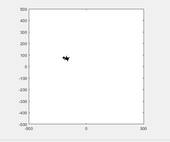
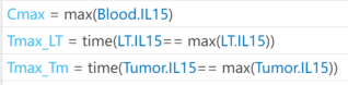
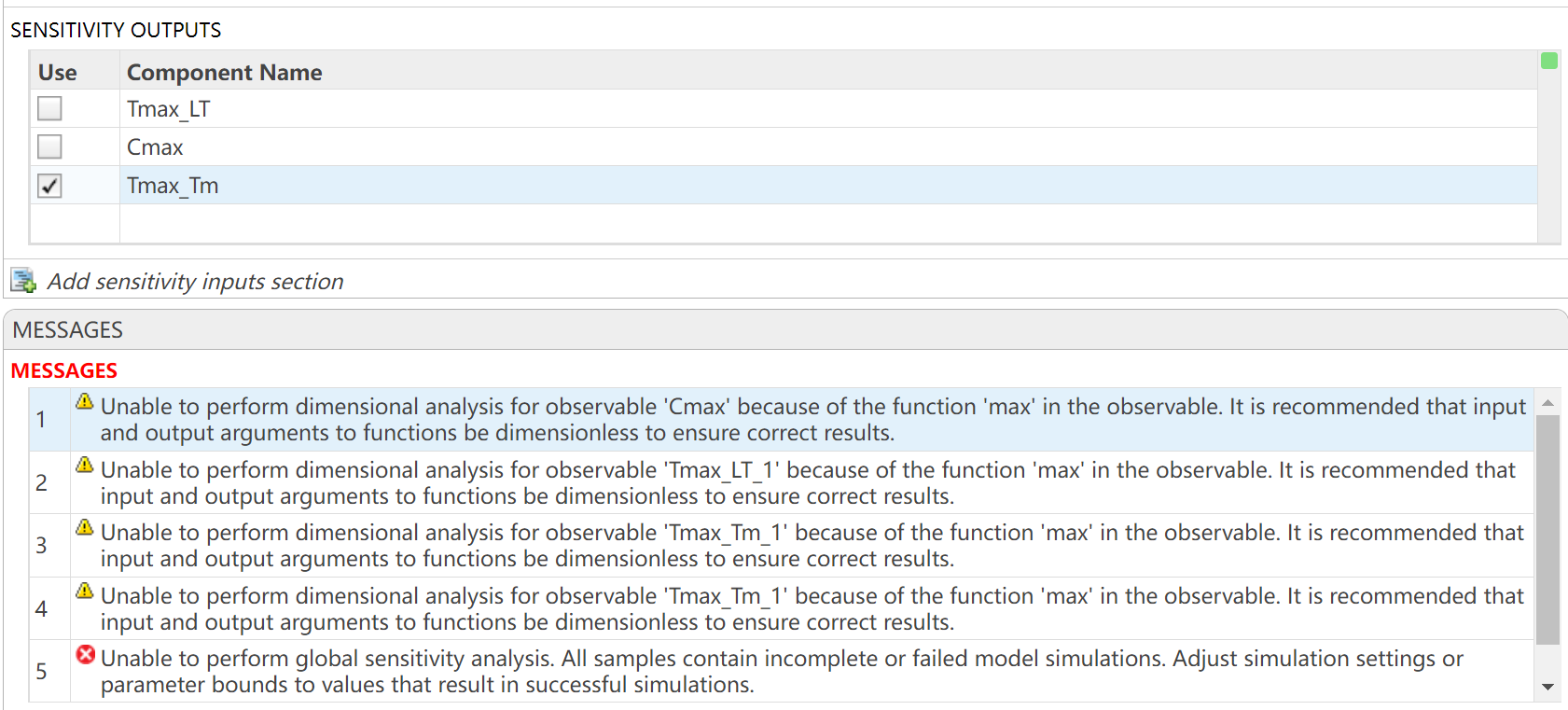
I want to observe the time (Tmax) to reach maximum drug concentration (Cmax) in my model. I have set up the OBSERVABLES as follows (figure1): Cmax = max(Blood.lL15); Tmax_LT = time(Conc_lL15_LT_nm == max(Conc_lL15_LT_nm)); Tmax_Tm = time(Conc_lL15_Tumor_nm == max(Conc_lL15_Tumor_nm)); After running the Sobol indices program for global sensitivity analysis, with inputs being some parameters and their ranges, the output for Cmax works, but there are some prompts, as shown in figure2. Additionally, when outputting Tmax, the program does not run successfully and reports some errors, as shown in figure2. How can I resolve the errors when outputting Tmax?
I like this problem by James and have solved it in several ways. A solution by Natalie impressed me and introduced me to a new function conv2. However, it occured to me that the numerous test for the problem only cover cases of square matrices. My original solutions, and Natalie's, did niot work on rectangular matrices. I have now produced a solution which works on rectangular matrices. Thanks for this thought provoking problem James.
I wanted to turn a Markdown nested list of text labels:
- A
- B
- C
- D
- G
- H
- E
- F
- Q
into a directed graph, like this:

Here is my blog post with some related tips for doing this, including text I/O, text processing with patterns, and directed graph operations and visualization.
The topic recently came up in a MATLAB Central Answers forum thread, where community members discussed how to programmatically control when the end user can close a custom app. Imagine you need to prevent app closure during a critical process but want to allow the end user to close the app afterwards. This article will guide you through the steps to add this behavior to your app.
A demo is attached containing an app with a state button that, when enabled, disables the ability to close the app.
Steps
1. Add a property that stores the state of the closure as a scalar logical value. In this example, I named the property closeEnabled. The default value in this example is true, meaning that closing is enabled. -- How to add a property to an app in app designer
properties (Access = private)
closeEnabled = true % Flag that controls ability to close app
end
2. Add a CloseRequest function to the app figure. This function is called any time there is an attempt to close the app. Within the CloseRequest function, add a condition that deletes the app when closure is enabled. -- How to add a CloseRequest function to an app figure in app designer
function UIFigureCloseRequest(app, event)
if app.closeEnabled
delete(app)
end
3. Toggle the value of the closeEnabled property as needed in your code. Imagine you have a "Process" button that initiates a process where it is crucial for the app to remain open. Set the closeEnabled flag to false (closure is disabled) at the beginning of the button's callback function and then set it to true at the end (closure is enabled).
function ProcessButtonPress(app, event)
app.closeEnabled = false;
% MY PROCESS CODE
app.closeEnabled = true;
end
Handling Errors: There is one trap to keep in mind in the example above. What if something in the callback function breaks before the app.closeEnabled is returned to true? That leaves the app in a bad state where closure is blocked. A pro move would be to use a cleanupObj to manage returning the property to true. In the example below, the task to return the closeEnabled property to true is managed by the cleanup object, which will execute that command when execution is terminated in the ProcessButtonPress function—whether execution was terminated by error or by gracefully exiting the function.
function ProcessButtonPress(app, event)
app.closeEnabled = false;
cleanupClosure = onCleanup(@()set(app,'closeEnabled',true));
% MY CODE
end
Force Closure: If the CloseRequest function is preventing an app from closing, here are a couple of ways to force a closure.
- If you have the app's handle, use delete(app) or close(app,'force'). This will also work on the app's figure handle.
- If you do not have the app's handle, you can use close('all','force') to close all figures or use findall(groot,'type','figure') to find the app's figure handle.
I have written, tested, and prepared a function with four subsunctions on my computer for solving one of the problems in the list of Cody problems in MathWorks in three days. Today, when I wanted to upload or copy paste the codes of the function and its subfunctions to the specified place of the problem of Cody page, I do not see a place to upload it, and the ability to copy past the codes. The total of the entire codes and their documentations is about 600 lines, which means that I cannot and it is not worth it to retype all of them in the relevent Cody environment after spending a few days. I would appreciate your guidance on how to enter the prepared codes to the desired environment in Cody.
Me: If you have parallel code and you apply this trick that only requires changing one line then it might go faster.
Reddit user: I did and it made my code 3x faster
Not bad for just one line of code!
Which makes me wonder. Could it make your MATLAB program go faster too? If you have some MATLAB code that makes use of parallel constructs like parfor or parfeval then start up your parallel pool like this
parpool("Threads")
before running your program.
The worst that will happen is you get an error message and you'll send us a bug report....or maybe it doesn't speed up much at all....
....or maybe you'll be like the Reddit user and get 3x speed-up for 10 seconds work. It must be worth a try...after all, you're using parallel computing to make your code faster right? May as well go all the way.
In an artificial benchmark I tried, I got 10x speedup! More details in my recent blog post: Parallel computing in MATLAB: Have you tried ThreadPools yet? » The MATLAB Blog - MATLAB & Simulink
Give it a try and let me know how you get on.
The GCD approach to identify rough numbers is a terribly useful one, well worth remembering. But at some point, I expect someone to notice that all work done with these massively large symbolic numbers uses only one of the cores on your computer. And, having spent so much money on those extra cores in your CPU, surely we can find a way to use them all? The problem is, computations done on symbolic integers never use more than 1 core. (Sad, unhappy face.)
In order to use all of the power available to your computer using MATLAB, you need to work in double precision, or perhaps int64 or uint64. To do that, I'll next search for primes among the family 3^n+4. In fact, they seem pretty common, at least if we look at the first few such examples.
F = @(n) sym(3).^n + 4;
F(0:16)
ans =
[5, 7, 13, 31, 85, 247, 733, 2191, 6565, 19687, 59053, 177151, 531445, 1594327, 4782973, 14348911, 43046725]
isprime(F(0:16))
ans =
1×17 logical array
1 1 1 1 0 0 1 0 0 1 1 0 0 0 0 0 0
Of the first 11 members of that sequence, 7 of them were prime. Naturally, primes will become less frequent in this sequence as we look further out. The members of this family grow rapidly in size. F(10000) has 4771 decimal digits, and F(100000) has 47712 decimal digits. We certainly don't want to directly test every member of that sequence for primality. However, what I will call a partial or incomplete sieve can greatly decrease the work needed.
Consider there are roughly 5.7 million primes less than 1e8.
numel(primes(1e8))
ans =
5761455
F(17) is the first member of our sequence that exceeds 1e8. So we can start there, since we already know the small-ish primes in this sequence.
roughlim = 1e8;
primes1e8 = primes(roughlim);
primes1e8([1 2]) = []; % F(n) is never divisible by 2 or 3
F_17 = double(F(17));
Fremainders = mod(F_17,primes1e8);
nmax = 100000;
FnIsRough = false(1,nmax);
for n = 17:nmax
if all(Fremainders)
FnIsRough(n) = true;
end
% update the remainders for the next term in the sequence
% This uses the recursion: F(n+1) = 3*F(n) - 8
Fremainders = mod(Fremainders*3 - 8,primes1e8);
end
sum(FnIsRough)
ans =
6876
These will be effectively trial divides, even though we use mod for the purpose. The result is 6876 1e8-rough numbers, far less than that total set of 99984 values for n. One thing of great importance is to recognize this sequence of tests will use an approximately constant time per test regardless of the size of the numbers because each test works off the remainders from the previous one. And that works as long as we can update those remainders in some simple, direct, and efficient fashion. All that matters is the size of the set of primes to test against. Remember, the beauty of this scheme is that while I did what are implicitly trial divides against 5.76 million primes at each step, ALL of the work was done in double precision. That means I used all 8 of the cores on my computer, pushing them as hard as I could. I never had to go into the realm of big integer arithmetic to identify the rough members in that sequence, and by staying in the realm of doubles, MATLAB will automatically use all the cores you have available.
The first 10 values of n (where n is at least 17), such that F(n) is 1e8-rough were
FnIsRough = find(FnIsRough);
FnIsRough(1:10)
ans =
22 30 42 57 87 94 166 174 195 198
How well does the roughness test do to eliminate composite members of this sequence?
isprime(F(FnIsRough(1:10)))
ans =
1×10 logical array
1 1 1 1 1 0 0 1 1 1
As you can see, 8 of those first few 1e8-rough members were actually prime, so only 2 of those eventual isprime tests were effectively wasted. That means the roughness test was quite useful indeed as an efficient but relatively weak pre-test for possible primality. More importantly it is a way to quickly eliminate those values which can be known to be composite.
You can apply a similar set of tests on many families of numbers. For example, repunit primes are a great case. A rep-digit number is any number composed of a sequence of only a single digit, like 11, 777, and 9999999999999.
However, you should understand that only rep-digit numbers composed of entirely ones can ever be prime. Naturally, any number composed entirely of the digit D, will always be divisible by the single digit number D, and so only rep-unit numbers can be prime. Repunit numbers are a subset of the rep-digit family, so numbers composed only of a string of ones. 11 is the first such repunit prime. We can write them in MATLAB as a simple expression:
RU = @(N) (sym(10).^N - 1)/9;
RU(N) is a number composed only of the digit 1, with N decimal digits. This family also follows a recurrence relation, and so we could use a similar scheme as was used to find rough members of the set 3^N-4.
RU(N+1) == 10*RU(N) + 1
However, repunit numbers are rarely prime. Looking out as far as 500 digit repunit numbers, we would see primes are pretty scarce in this specific family.
find(isprime(RU(1:500)))
ans =
2 19 23 317
There are of course good reasons why repunit numbers are rarely prime. One of them is they can only ever be prime when the number of digits is also prime. This is easy to show, as you can always factor any repunit number with a composite number of digits in a simple way:
1111 (4 digits) = 11*101
111111111 (9 digits) = 111*1001001
Finally, I'll mention that Mersenne primes are indeed another example of repunit primes, when expressed in base 2. A fun fact: a Mersenne number of the form 2^n-1, when n is prime, can only have prime factors of the form 1+2*k*n. Even the Mersenne number itself will be of the same general form. And remember that a Mersenne number M(n) can only ever be prime when n is itself prime. Try it! For example, 11 is prime.
Mn = @(n) sym(2).^n - 1;
Mn(11)
ans =
2047
Note that 2047 = 1 + 186*11. But M(11) is not itself prime.
factor(Mn(11))
ans =
[23, 89]
Looking carefully at both of those factors, we see that 23 == 1+2*11, and 89 = 1+8*11.
How does this help us? Perhaps you may see where this is going. The largest known Mersenne prime at this date is Mn(136279841). This is one seriously massive prime, containing 41,024,320 decimal digits. I have no plans to directly test numbers of that size for primality here, at least not with my current computing capacity. Regardless, even at that realm of immensity, we can still do something.
If the largest known Mersenne prime comes from n=136279841, then the next such prime must have a larger prime exponent. What are the next few primes that exceed 136279841?
np = NaN(1,11); np(1) = 136279841;
for i = 1:10
np(i+1) = nextprime(np(i)+1);
end
np(1) = [];
np
np =
Columns 1 through 8
136279879 136279901 136279919 136279933 136279967 136279981 136279987 136280003
Columns 9 through 10
136280009 136280051
The next 10 candidates for Mersenne primality lie in the set Mn(np), though it is unlikely that any of those Mersenne numbers will be prime. But ... is it possible that any of them may form the next Mersenne prime? At the very least, we can exclude a few of them.
for i = 1:10
2*find(powermod(sym(2),np(i),1+2*(1:50000)*np(i))==1)
end
ans =
18 40 64
ans =
1×0 empty double row vector
ans =
2
ans =
1×0 empty double row vector
ans =
1×0 empty double row vector
ans =
1×0 empty double row vector
ans =
1×0 empty double row vector
ans =
1×0 empty double row vector
ans =
1×0 empty double row vector
ans =
2
Even with this quick test which took only a few seconds to run on my computer, we see that 3 of those Mersenne numbers are clearly not prime. In fact, we already know three of the factors of M(136279879), as 1+[18,40,64]*136279879.
You might ask, when is the MOD style test, using a large scale test for roughness against many thousands or millions of small primes, when is it better than the use of GCD? The answer here is clear. Use the large scale mod test when you can easily move from one member of the family to the next, typically using a linear recurrence. Simple such examples of this are:
1. Repunit numbers
General form: R(n) = (10^n-1)/9
Recurrence: R(n+1) = 10*R(n) + 1, R(0) = 1, R(1) = 11
2. Fibonacci numbers.
Recurrence: F(n+1) = F(n) + F(n-1), F(0) = 0, F(1) = 1
3. Mersenne numbers.
General form: M(n) = 2^n - 1
Recurrence: M(n+1) = 2*M(n) + 1
4. Cullen numbers, https://en.wikipedia.org/wiki/Cullen_number
General form: C(n) = n*2^n + 1
Recurrence: C(n+1) = 4*C(n) + 4*C(n-1) + 1
5. Hampshire numbers: (My own choice of name)
General form: H(n,b) = (n+1)*b^n - 1
Recurrence: H(n+1,b) = 2*b*H(n-1,b) - b^2*H(n-2,b) - (b-1)^2, H(0,b) = 0, H(1,b) = 2*b-1
6. Tin numbers, so named because Sn is the atomic symbol for tin.
General form: S(n) = 2*n*F(n) + 1, where F(n) is the nth Fibonacci number.
Recurrence: S(n) = S(n-5) + S(n-4) - 3*S(n-3) - S(n-2) +3*S(n-1);
To wrap thing up, I hope you have enjoyed this beginning of a journey into large primes and non-primes. I've shown a few ways we can use roughness, first in a constructive way to identify numbers which may harbor primes in a greater density than would otherwise be expected. Next, using GCD in a very pretty way, and finally by use of MOD and the full power of MATLAB to test elements of a sequence of numbers for potential primality.
My next post will delve into the world of Fermat and his little theorem, showing how it can be used as a stronger test for primality (though not perfect.)
Yes, some readers might now argue that I used roughness in a crazy way in my last post, in my approach to finding a large twin prime pair. That is, I deliberately constructed a family of integers that were known to be a-priori rough. But, suppose I gave you some large, rather arbitrarily constructed number, and asked you to tell me if it is prime? For example, to pull a number out of my hat, consider
P = sym(2)^122397 + 65;
floor(vpa(log10(P) + 1))
36846 decimal digits is pretty large. And in fact, large enough that sym/isprime in R2024b will literally choke on it. But is it prime? Can we efficiently learn if it is at least not prime?
A nice way to learn the roughness of even a very large number like this is to use GCD.
gcd(P,prod(sym(primes(10000))))
If the greatest common divisor between P and prod(sym(primes(10000))) is 1, then P is NOT divisible by any small prime from that set, since they have no common divisors. And so we can learn that P is indeed fairly rough, 10000-rough in fact. That means P is more likely to be prime than most other large integers in that domain.
gcd(P,prod(sym(primes(100000))))
However, this rather efficiently tells us that in fact, P is not prime, as it has a common factor with some integer greater than 1, and less then 1e5.
I suppose you might think this is nothing different from doing trial divides, or using the mod function. But GCD is a much faster way to solve the problem. As a test, I timed the two.
timeit(@() gcd(P,prod(sym(primes(100000)))))
timeit(@() any(mod(P,primes(100000)) == 0))
Even worse, in the first test, much if not most of that time is spent in merely computing the product of those primes.
pprod = prod(sym(primes(100000)));
timeit(@() gcd(P,pprod))
So even though pprod is itself a huge number, with over 43000 decimal digits, we can use it quite efficiently, especially if you precompute that product if you will do this often.
How might I use roughness, if my goal was to find the next larger prime beyond 2^122397? I'll look fairly deeply, looking only for 1e7-rough numbers, because these numbers are pretty seriously large. Any direct test for primality will take some serious time to perform.
pprod = prod(sym(primes(10000000)));
find(1 == gcd(sym(2)^122397 + (1:2:199),pprod))*2 - 1
2^122397 plus any one of those numbers is known to be 1e7-rough, and therefore very possibly prime. A direct test at this point would surely take hours and I don't want to wait that long. So I'll back off just a little to identify the next prime that follows 2^10000. Even that will take some CPU time.
What is the next prime that follows 2^10000? In this case, the number has a little over 3000 decimal digits. But, even with pprod set at the product of primes less than 1e7, only a few seconds were needed to identify many numbers that are 1e7-rough.
P10000 = sym(2)^10000;
k = find(1 == gcd(P10000 + (1:2:1999),pprod))*2 - 1
k =
Columns 1 through 8
15 51 63 85 165 171 177 183
Columns 9 through 16
253 267 273 295 315 421 427 451
Columns 17 through 24
511 531 567 601 603 675 687 717
Columns 25 through 32
723 735 763 771 783 793 795 823
Columns 33 through 40
837 853 865 885 925 955 997 1005
Columns 41 through 48
1017 1023 1045 1051 1071 1075 1095 1107
Columns 49 through 56
1261 1285 1287 1305 1371 1387 1417 1497
Columns 57 through 64
1507 1581 1591 1593 1681 1683 1705 1771
Columns 65 through 69
1773 1831 1837 1911 1917
Among the 1000 odd numbers immediately following 2^10000, there are exactly 69 that are 1e7-rough. Every other odd number in that sequence is now known to be composite, and even though we don't know the full factorization of those 931 composite numbers, we don't care in the context as they are not prime. I would next apply a stronger test for primality to only those few candidates which are known to be rough. Eventually after an extensive search, we would learn the next prime succeeding 2^10000 is 2^10000+13425.
In my next post, I show how to use MOD, and all the cores in your CPU to test for roughness.