Results for
AI Skills for deployment of a MATLAB Live Script as a free iOS App
My Live Script to mobile-phone app conversion in 20-minutes-ish, with AI describes the conversion of a MATLAB Live Script to an iOS App running in a simulator. The educational app is now available on the App Store as Newton’s Cradle, Unbound. It’s free, ad-free, and intended to interest students of physics and the curious.
I provide below a Claude AI-generated overview of the deployment process, and I attach in standard Markdown format two related Claude-generated skill files. The Markdown files can be rendered in Visual Studio Code. (Change .txt to .md.) I used my universal agentic AI setup, but being totally unfamiliar with the Apple app submission process, I walked through the many steps slowly, with continuous assistance over the course of many hours. If I were to do this again, much could be automated.
There were several gotcha’s. For example, simulator screenshots for both iPhone and iPad must be created of a standard size, not documented well by APPLE but known to the AI, and with a standard blessed time at the top, not the local time. Claude provided a bash command to eliminate those when simulating. A privacy policy on an available website and contact information are needed. Claude helped me design and create a fun splash page and to deploy it on GitHub. The HTML was AI-generated and incorporated an Apple-approved icon (Claude helped me go find those), an app-specific icon made by Claude based on a prompt. We added a link to a privacy policy page and a link to a dedicated Google support email account created for the App - Claude guided me through that, too. Remarkably, the App was approved and made available without revision.
Documentation Overview
1. iOS App Store Submission Skill
Location: SKILL-ios-store-submission.md
This is a comprehensive guide covering the complete App Store submission workflow:
• Prerequisites (Developer account, Xcode, app icon, privacy policy)
• 12-step process from certificate creation through final submission
• Troubleshooting for common errors (missing icons, signing issues, team not appearing)
• Screenshot requirements and capture process
• App Store Connect metadata configuration
• Export compliance handling
• Apple trademark guidelines
• Complete checklists and glossary
• Reference URLs for all Apple portals
Key sections: Certificate creation, Xcode signing setup, app icon requirements (1024x1024 PNG), screenshot specs, privacy policy requirements, build upload process, and post-submission status tracking.
2. GitHub Pages Creation Skill
Location: github-pages/SKILL.md
This documents the GitHub Pages setup workflow using browser automation:
• 5-step process to create and deploy static websites
• HTML templates for privacy policies (iOS apps with no data collection)
• Browser automation commands (tabs_context_mcp, navigate, form filling)
• Enabling GitHub Pages in repository settings
• Troubleshooting common deployment issues
• Output URL format: https://username.github.io/repo-name/
Key templates: Privacy policy HTML with proper Apple-style formatting, contact information structure, and responsive CSS.
These files capture the complete technical process, making it easy to:
• Submit future iOS apps without re-discovering the steps
• Help others through the submission process
• Reference specific troubleshooting solutions
• Reuse HTML templates for other apps' privacy policies
I used Claude Code along with MATLAB's MCP server to develop this animation that morphs between the MATLAB membrane and a 3D heart. Details at Coding a MATLAB Valentine animation with agentic AI » The MATLAB Blog - MATLAB & Simulink
Show me what you can do!
If you share code, may I suggest putting it in a GitHib repo and posting the link here rather than posting the code directly in the forum? When we tried a similar exercise on Vibe-coded Christmas trees, we posted the code directly to a single discussion thread and quickly brought the forum software to its knees.

Over the past few days I noticed a minor change on the MATLAB File Exchange:
For a FEX repository, if you click the 'Files' tab you now get a file-tree–style online manager layout with an 'Open in new tab' hyperlink near the top-left. This is very useful:
If you want to share that specific page externally (e.g., on GitHub), you can simply copy that hyperlink. For .mlx files it provides a perfect preview. I'd love to hear your thoughts.
EXAMPLE:
🤗🤗🤗
New release! MATLAB MCP Core Server v0.5.0 !
The latest version introduces MATLAB nodesktop mode — a feature that lets you run MATLAB without the Desktop UI while still sending outputs directly to your LLM or AI‑powered IDE.
Here's a screenshot from the developer of the feature.
Check out the release here Releases · matlab/matlab-mcp-core-server
Hi everyone,
I'm a biomedical engineering PhD student who uses MATLAB daily for medical image analysis. I noticed that Claude often suggests MATLAB+Python workarounds or thirdparty toolboxesfor tasks that MATLAB can handle natively, or recommends functions that were deprecated several versions ago.
To address this, I created a set of skills that help Claude understand what MATLAB can actually do—especially with newer functions and toolbox-specific capabilities. This way, it can suggest pure MATLAB solutions instead of mixing in Python or relying on outdated approaches.
What I Built
The repo covers Medical Imaging, Image Processing, Deep Learning, Stats/ML, and Wavelet toolbox based skills. I tried my best to verify everything against R2025b documentation.
Feedback Welcome
If you try them out, I'd like to hear how it goes. And if you run into errors or have ideas, feel free to create an issue. If you find them useful, a "Star" on the repo would be appreciated. This is my first time putting something like this out there, so any feedback helps.
Also, if anyone is interested in collaborating on an article for the MathWorks blog, I'd be happy to volunteer and collaborate on this topic or related topics together!
I look forward to hearing from you....
Thanks!
I recently created a short 5-minute video covering 10 tips for students learning MATLAB. I hope this helps!
In 2025, we saw the growing impact of GenAI on site traffic and user behavior across the entire technical landscape. Amid all this change, MATLAB Central continued to stand out as a trusted home for MATLAB and Simulink users. More than 11 million unique visitors in 2025 came to MATLAB Central to ask questions, share code, learn, and connect with one another.
Let’s celebrate what made 2025 memorable across three key areas: people, content, and events.
People
In 2025, nearly 20,000 contributors participated across the community. We’d like to spotlight a few standout contributors:
- @Sam Chak earned the Most Accepted Answers Badge for both 2024 and 2025. Sam is a rising star in MATLAB Answers with 2,000+ answers and 1,000+ votes.
- @Rodney Tan has been actively contributing files to File Exchange. In 2025, his submissions got almost 20,000 downloads!
- @Dyuman Joshi was recognized as a top contributor on both Cody and Answers. Many may not know that Dyuman is also a Cody moderator, doing tremendous behind-the-scenes moderation work to keep the platform running smoothly.
- A warm welcome to @Steve Eddins, who joined the Community Advisory Board. Steve brings a unique perspective as a former MathWorker and long-time top community contributor.
- Congratulations to @Walter Roberson on reaching 100 followers! MATLAB Central thrives on people-to-people connections, and we’d love to see even more of these relationships grow.
Of course, there are many contributors we didn’t mention here—thank you all for your outstanding contributions and for making the community what it is.
Content
Our high-quality community content not only attracts users but also helps power the broader GenAI ecosystem.
Popular Blog Post & File Exchange Submission
- Zoomed Axes, submitted by @Caleb Thomas, enables zoomed-in views of selected regions in a plot.This submission was featured in the Pick of the Week blog post, “MATLAB Zoomed Axes: Showing zoomed-in regions of a 2D plot,” which generated 5,000 views in just one month.
Popular Discussion Post
- What did MATLAB/Simulink users wait for most in 2025? It's R2025a! “Where is MATLAB R2025a?” became the most-viewed discussion post, with 10,000 views and 30 comments. Thanks for your patience — MATLAB R2025a turned out to be one of the biggest releases we’ve ever delivered.
Most Viewed Question
- “How do I create a for loop in MATLAB?” was the most-viewed community question of the year. It’s a fun reminder that even as MATLAB evolves, the basics remain essential — and always in demand.
Most Voted Poll
- “Did you know there is an official MATLAB certification?”, created by @goc3, was the most-voted poll of 2025.While 50% of respondents voted “No”, it’s exciting to see 3% are certified MATLAB Professionals. Will you be one of them in 2026?
Events
The Cody Contest 2025 brought teams together to tackle challenging but fun Cody problems. During the contest:
- 20,000+ solutions were submitted
- 20+ tips & tricks articles were shared by top players
While the contest has ended, you can still challenge yourself with the fun contest problem group. If you get stuck, the tips & tricks articles are a great resource—and you’ll be amazed by the creativity and skill of the contributors.
Thank you for being part of an incredible 2025. Your curiosity, generosity, and expertise are what make MATLAB Central a trusted home for millions—and we look forward to learning and growing together in 2026.
AI-assisted software development moves pretty fast! I recently noticed everyone in the AI community talking about a Simpson's character. I originally thought it was some joke-meme that I didn't understand but it turns out to be an AI development methodology claude-code/plugins/ralph-wiggum/README.md at main · anthropics/claude-code
I noticed that @Toshiaki Takeuchi mentioned it in my recent interview of him over at The MATLAB blog https://blogs.mathworks.com/matlab/2026/01/26/matlab-agentic-ai-the-workflow-that-actually-works/
Has anyone here tried this yet?
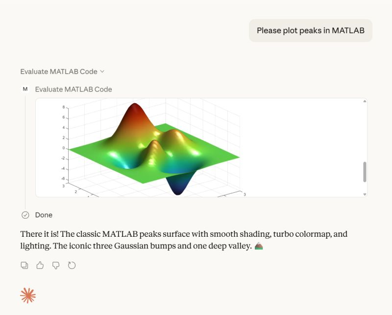
I gave it a try on my mac mini m4. I'm speechless 🤯
Educators in mid 2025 worried about students asking an AI to write their required research paper. Now, with agentic AI, students can open their LMS with say Comet and issue the prompt “Hey, complete all my assignments in all of my courses. Thanks!” Done. Thwarting illegitimate use of AIs in education without hindering the many legitimate uses is a cat-and-mouse game and burgeoning industry.
I am actually more interested in a new AI-related teaching and learning challenge: how one AI can teach another AI. To be specific, I have been discovering with Claude macOS App running Opus 4.5 how to school LM Studio macOS App running a local open model Qwen2.5 32B in the use of MATLAB and other MCP services available to both apps, so, like Claude, LM Studio can operate all of my MacOS apps, including regular (Safari) and agentic (Comet or Chrome with Claude Chrome Extension) browsers and other AI Apps like ChatGPT or Perplexity, and can write and debug MATLAB code agentically. (Model Context Protocol is the standardized way AI apps communicate with tools.) You might be playing around with multiple AIs and encountering similar issues. I expect the AI-to-AI teaching and learning challenge to go far beyond my little laptop milieu.
To make this concrete, I offer the image below, which shows LM Studio creating its first Excel spreadsheet using Excel macOS app. Claude App in the left is behind the scenes there updating LM Studio's context window.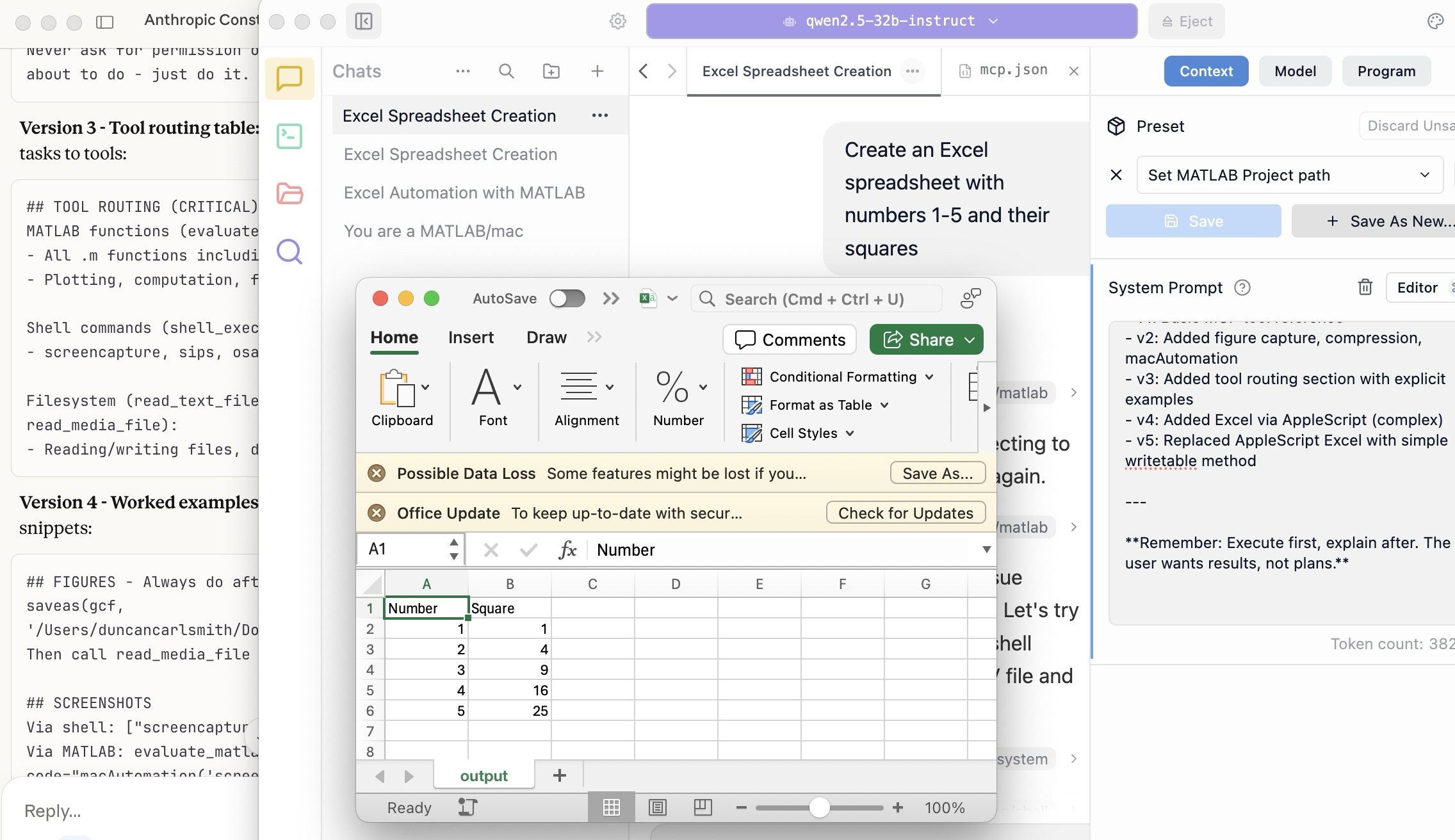
A teacher needs to know something but is at best a guide and inspiration, never a total fount of knowedge, especially today. Working first with Claude alone over the last few weeks to develop skills has itself been an interesting collaborative teaching and learning experience. We had to figure out how to use our MATLAB and other MCP services with various macOS services and some ancillary helper MATLAB functions with hopefully the minimal macOS permissions needed to achieve the desired functionality. Loose permissions allow the AI to access a wider filesystem with shell access, and, for example, to read or even modify an application’s preferences and permissions, and to read its state variables and log files. This is valuable information to an AI in trying to successfully operate an application to achieve some goal. But one might not be comfortable being too permissive.
The result of this collaboration was an expanding bag of tricks: Use AppleScript for this app, but a custom Apple shortcut for this other app; use MATLAB image compression of a screenshot (to provide feedback on the state and results) here, but if MATLAB is not available, then another slower image processing application; use cliclick if an application exposes its UI elements to the Accessibility API, but estimate a cursor relocation from a screenshot of one or more application windows otherwise. Texting images as opposed to text (MMS v SMS) was a challenge. And it’s going to be more complex if I use a multi-monitor setup.
Having satisfied myself that we could, with dedication, learn to operate any app (though each might offer new challenges), I turned to training another AI, similarly empowered with MCP services, to do the same, and that became an interesting new challenge. Firstly, we struggled with the Perplexity App, configured with identical MCP and other services, and found that Perplexity seems unable to avail itself of them. So we turned to educating LM Studio, operating a suite of models downloaded to my laptop.
An AI today is just a model trained in language prediction at some time. It is task-oriented and doesn’t know what to do in a new environment. It needs direction and context, both general and specific. AI’s now have web access to current web information and, given agentic powers, can on their own ask other AI’s for advice. They are quick-studies.
The first question in educating LM Studio was which open model to use. I wanted one that matched my laptop hardware - an APPLE M1 Max (10-core) CPU with integrated 24-core GPU with 64 GB shared memory- and had smarts comparable to Claude’s Opus 4.5 model. We settled on Mistral-Nemo-Instruct 2407 (12B parameters, ~7GB) and got it to the point where it could write and execute a MATLAB code to numerically integrate the equations of motion for a pendulum. Along the way, delving into the observation that the Mistral model's pendulum amplitude was drifting, I learned from Claude about symplectic integration. A teacher is always learning. Learning makes teaching fun.
But, long story short, we learned in the end that this model in this context was unable to see logical errors in code and fix them like Claude. So we tried and settled on some different models: Qwen 2.5 7B Instruct for speed, or Qwen 2.5 32B Instruct for more complex reasoning. The preliminary results looks good!
Our main goal was to teach a model how to use the unusual MCP and linked services at its disposal, starting from zero, and as you might educate a beginning student in physics or whatever through exercises and direct experience. Along the way, in teaching for the first time, we developed a kind of nascent curriculum strategy just to introduce the model to its new capabilities. Allow me to let Claude summarize just to give you a sense. There will not be a test on this material.
The Bootstrapping Process
Phase 1: Discovery of the Problem
The Qwen/Mistral models would describe what they would do rather than execute tools. They'd output JSON text showing what a tool call would look like, rather than actually triggering the tool. Or they'd say "I would use the evaluate_matlab_code tool to..." without doing it.
Phase 2: Explicit Tool Naming
First fix - be explicit in prompts:
Use the evaluate_matlab_code tool to run this code...
Instead of:
Run this MATLAB script...
This worked, but required the user to know tool names.
Phase 3: System Prompt Engineering
We iteratively built up a system prompt (Context tab in LM Studio) that taught the model:
Version 1 - Basic path:
When using MATLAB tools, always use /Users/username/Documents/MATLAB
as the project_path unless the user specifies otherwise.
Version 2 - Forceful execution:
IMPORTANT: When you need to use a tool, execute it immediately.
Do not describe the tool call or show JSON - just call the tool directly.
Never ask for permission or explain what you're about to do - just do it.
Version 3 - Tool routing table:
Added explicit mapping of tasks to tools:
## TOOL ROUTING (CRITICAL)
MATLAB functions (evaluate_matlab_code):
- All .m functions including macAutomation()
- Plotting, computation, file I/O
Shell commands (shell_execute):
- screencapture, sips, osascript, open, say...
Filesystem (read_text_file, write_file, read_media_file):
- Reading/writing files, displaying images
Version 4 - Worked examples:
Added concrete code snippets:
## FIGURES - Always do after plotting:
saveas(gcf, '/Users/username/Documents/MATLAB/LMStudio/latest_figure.png');
Then call read_media_file to display it.
## SCREENSHOTS
Via shell: ["screencapture", "-x", "output.png"]
Via MATLAB: evaluate_matlab_code with code="macAutomation('screenshot','screen')"
Version 5 - Physics patterns:
## PHYSICS - Use Symplectic Integration
omega(i) = omega(i-1) - (g/L)*sin(theta(i-1))*dt;
theta(i) = theta(i-1) + omega(i)*dt; % Use NEW omega
NOT: theta(i-1) + omega(i-1)*dt % Forward Euler drifts!
Phase 4: Prompt Phrasing for Smaller Models
Discovered that 7B-12B models needed "forceful" phrasing:
Execute now: Use evaluate_matlab_code to run this code...
And recovery prompts when they stalled:
Proceed with the tool call
Execute the fix now
Phase 5: Saving as Preset
Along the way, we accumulated various AI-speak directions and ultimately the whole context as a Preset in LM Studio, so it persists across sessions.
Now the trend in the AI industry is to develop and then share or publish “skills” rather like the Preset in a standard markdown structure, like CliffsNotes for AI. My notes/skills won't fit your environment and are evolving. They may appear biased against French models and too pro-Anthropic, and so on. We may need to structure AI education and AI specialization going forward in innovative ways, but may face familiar issues. Some AIs can be self-taught given the slightest nudge. Others less resource priviledged will struggle in their education and future careers. Some may even try to cheat and face a comeuppance.
The next step is to see if Claude can delegate complex tasks to local models, creating a tiered system where a frontier model orchestrates while cheaper models execute.
Anthropic has just announced Claude’s Constitution to govern Claude’s behavior in anticipation of a continued ramp-up to AGI abilities. Amusing me just now, just as this constitution was announced, I was encountering a wee moral dilemma myself with Claude.
Claude and I were trying to transfer all of Claude’s abilities and knowledge for controlling macOS and iPhone apps in my setup (See A universal agentic AI for your laptop and beyond) to the Perplexity App. My macOS Perplexity App is configured with the full suite of MCP services available to my Claude App, but I hadn’t yet exercised these with Perplexity App. Oddly, all but Playwright failed to work despite our many experiments and searches for information at Perplexity and elsewhere.
I suspect that Perplexity built into the macOS app all the hooks for MCP, but became gun-shy for security reasons and enforced constraints so none of its models (not even the very model Claude App was running) can execute MCP-related commands, oddly except those for PlayWright. The Perplexity App even offers a few of its own MCP connectors, but these are also non-functional. It is possible we missed something. These limitations appear to be undocumented.
Pulling our hair out, Claude and I were wondering how such constraints might be implemented, and Claude suggested an experiment and then a possible workaround. At that point, I had to pause and say, “No, we are not going there.” No, I won’t tell you the suggested workaround. No, we didn’t try it. Tempting in the moment, but no.
Be safe. And be a good person. Don’t let your enthusiasm reign unbridled.
Disclosure: The author has no direct financial interest in Anthropic, and loves Perplexity App and Comet too, but his son (a philosopher by training) is the lead author on this draft of the Constitution, and overuses the phrase “broadly speaking” in my opinion.
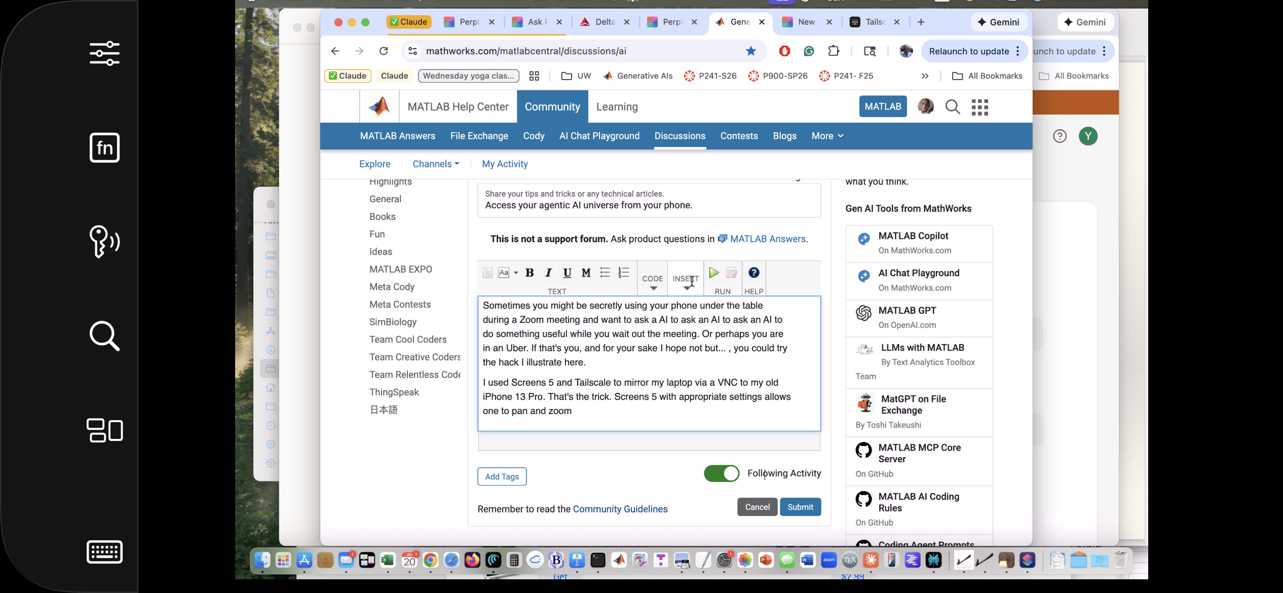
Sometimes you might be secretly using your phone under the table, or stuck in traffic in an Uber, and want to ask a AI to ask an AI to ask an AI to do something useful. If that's you (and for your sake I hope not but... ), you could try the hack illustrated here.
This article illustrates experiments with APPLE products and uses Claude (Anthropic.com) but is not an endorsement of any AI or mobile phone or computer system vendor. Similar things could be done by hooking together other products and services. My setup is described in A universal agentic AI for your laptop and beyond. Please be aware of the security risks in granting any AI access to your systems.
I have now used Screens 5 and tailscale to mirror my laptop via a VNC to my old iPhone 13 Pro. That's the trick. With appropriate settings Screens, allows one to pan and zoom in order to operate the otherwise-too-tiny laptop controls. An AI can help you install and configure thtese products.
The image below is an iPhone screensnap of the Screens iPhone App showing my laptop browser while editing this article. I could be writing this article on my phone manually. I could be operating an AI to write this article. But just FYI, I'm not. :)
Below is a screensnap of APPLE KeyNote. On the slide is a screenshot of iPhone Screen-view of the laptop itself. Via Screens on iPhone, I had asked Claude App on my laptop to open a Keynote presentation on my laptop concerning AI. The Keynote slide is about using iPhone to ask Claude App to operate an AI at Huggface. Or something like that - I'm totally lost. Aren't you?

Of course, you can operate Claude App or Perplexity App on iPhone but, as of this writing, Claude Chrome Extension and Perplexity Comet are not yet available for iPhone, limiting agentic use to your laptop. And these systems can not access your native laptop applications and your native AI models so I think Screens or an equivalent may be the only way at present to bring all this functionality to your phone.
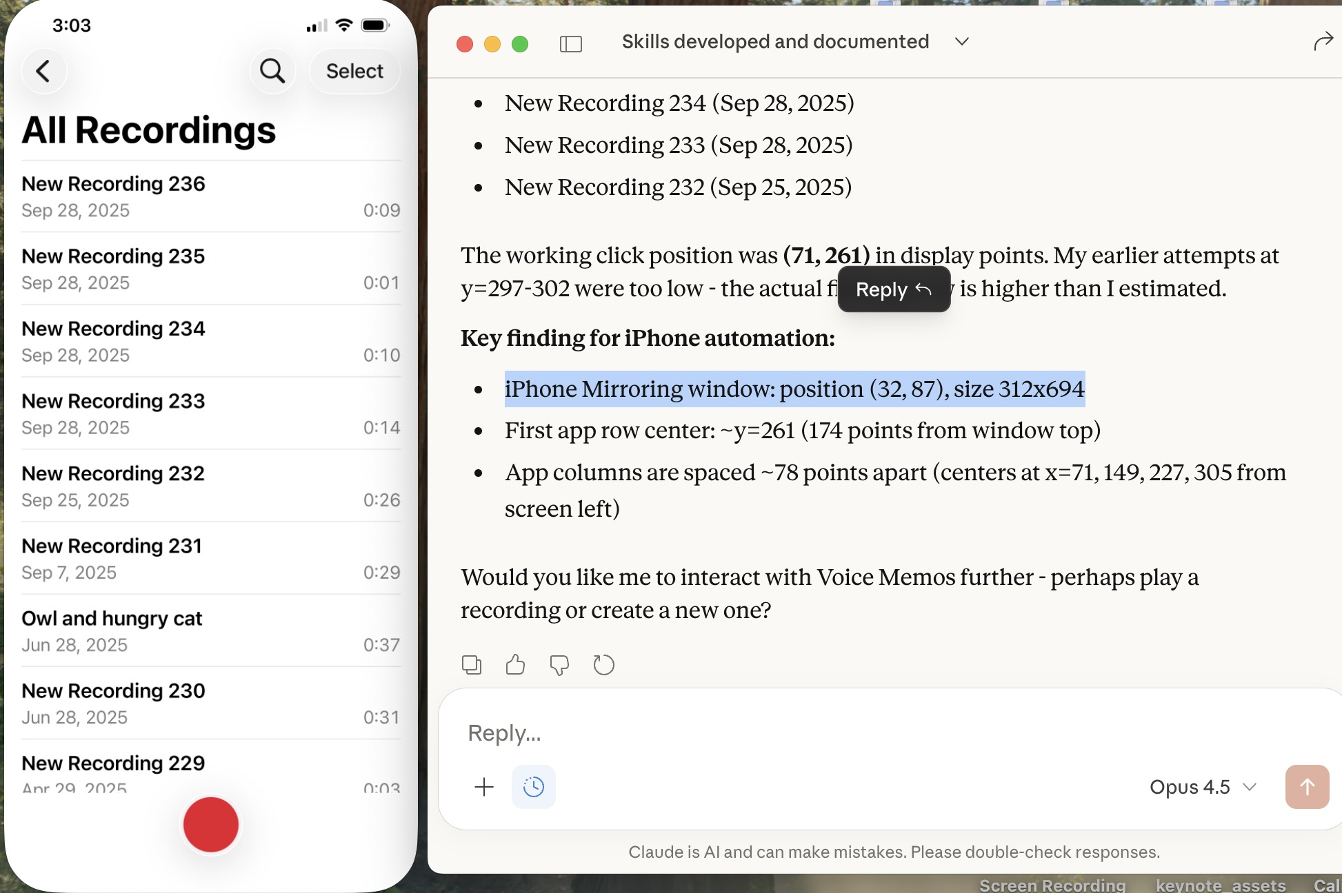
Sweet, but can I operate my iPhone agentically? Um,..., actually yes. The trick is to turn on iPhone mirroring so the iPhone appears on your laptop with all of the iPhone buttons clickable using the laptop touch pad. And a local AI is pretty good at clicking using clicclic and other tricks. It can be a little painful the first time to discover how to perform such operations and the tricks are best remembered as AI skills.
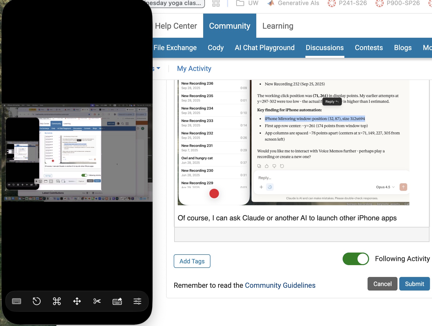
Below is a screensnap of my laptop showing the mirrored iPhone on the left. On the right is my Claude Desktop App. I asked Claude to launch Voice Memos and Claude developed a method to do this. We are ready to play a recording stored there (it will be heard through my laptop speaker) or edit it or email it to someone, or whatever. If you thought to initiate a surreptious audio recording or camera image, be aware that APPLE has disabled those functionalities.
Of course, I can ask Claude (or another AI) to launch other iPhone apps, even Screens app as you can see below. This is a screensnap of my laptop with iPhone mirroring and with iPhone Screens App launched on the phone showing the laptop screen as I write this article, or something like that. ;)
Next, let me use Claude desktop app with iPhone mirroring to switch to iPhone Claude App or iPhone Perplexity App and... Nevermind. I think the point has been made well enough. The larger lesson perhaps is to consider how agentic AIs can thusly and otherwise operate one's personal the internet of things, say check if my garage door is closed etc. Have fun. Be safe.
I was wondering yesterday if an AI could help me conquer something I had considered to difficult to bother with, namely creating a mobile-phone app. I had once ages ago played with Xcode on my laptop, leanrng not only would I have to struggle with the UI but learn Swift to boot, plus Xcode, so...neah. Best left to specialists.
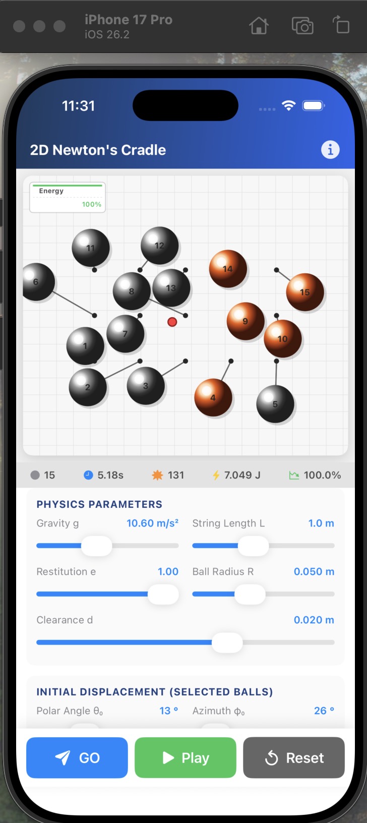
This article describes an experiment in AI creation of an HTML5 prototype and then a mobile-phone app, based on an educational MATLAB Live Script. The example target script is Two-dimensional Newton Cradles, a fun Live Script for physics students by the author. (You can check out my other scripts at File Exchange here.) The target script involves some nontrivial collisional dynamics but uses no specialized functions. The objective was to create a mobile phone app that allows the user to exercise interactive controls similar to the slider controls in the Live Script but in an interactive mobile-phone-deployed simulation. How did this experiment go? A personal best!!
Using the AI setup described in A universal agentic AI for your laptop and beyond, Claude AI was directed to first study the Live Script and then to invent an HTML5 prototype as described in Double Pendulum Chaos Explorer: From HTML5 Prototype to MATLAB interactive application with AI. (All in one prompt.) Claude was then directed to convert the HTML5 to Swift in a project structure and to operate Xcode to generate an iOS app. The use of Claude (Anthropic) and iOS (APPLE) does not constitute endorsement of these products. Similar results are possible with other AIs and operating systems.
Here is the HTML5 version in a browser:

The HTML5 creation was the most lengthy part of the process. (Actually, documenting this is the most lengthy part!) The AI made an initial guess as to what interactive controls to support. I had to test the HTML5 product and say a few things like "You know, I want to include controls for the number of pendulums and for the pendulum lattice shape and size too, OK?"
When the HTML5 seemed good, I asked for suggestions for how best to fit that to a tiny mobile phone display screen and make some selections of options provided. I was sweating at that point, thinking "This is not going to go well..." Actually, I had already done a quick experiment to build a very simple app to put Particle Data Group information into an app and that went swimmingly well. The PDG had already tried submitting such an app to APPLE and been dismissed as trying to publish a book so I wasn't going to pursue it. But THAT app just had to display some data, not calculate anything.
It did go well. There was one readily fixed error in the build, then voila. I added some tweaks including an information page. Here is the iPhone app in the simulator.
The File Exchange package Live Script to Mobile-Phone App Conversion with AI contains: 1) the HTML5 prototype which may be compared to the original Live Script, 2) a livescript-2-ios-skill that may be imported into any AI to assist in replicating the process, and 3) related media files. Have fun out there! Bear with me as I sort out what zip uploads are permitted there. It seems a zip folder structure is not!
I see many people are using our new MCP Core Sever to do amazing things with MATLAB and AI. Some people are describing their experiements here (e.g. @Duncan Carlsmith) and on LinkedIn (E.g. Sergiu-Dan Stan and Toshi Takeuchi) and we are getting lots of great feedback.Some of that feedback has been addressed in the latest release so please update your install now.
MATLAB MCP Core Server v0.4.0 has been released on public GitHub:
Release highlights:
- Added Plain Text Live Code Guidelines MCP resource
- Added MCP Annotations to all tools
We encourage you to try this repository and provide feedback. If you encounter a technical issue or have an enhancement request, create an issue https://github.com/matlab/matlab-mcp-core-server/issues
Wouldn’t it be great if your laptop AI app could convert itself into an agent for everything? I mean for your laptop and for the entire web? Done.
Setup
My setup is a MacBook with MATLAB and various MCP servers. I have several equivalent Desktop AI apps configured. I will focus on the use of Claude App but fully expect Perplexity App to behave similarly. See How to set up and use AI Desktop Apps with MATLAB and MCP servers.
Warning: My setup grants Claude access to various macOS system services and may have unforeseen consequences. Try this entirely at your own risk, and carefully until comfortable.
My MacOS permissions include
Settings=>Privacy & Security=> Accessibility
where matlab-mcp-core-server and MATLAB enabled, and in
Settings=>Privacy & Security=> Automation,
matlab-mcp-core-server has been enabled to access on a case-by-case basis the applications Comet, Messages, Safari, Terminal, Keynote, Mail, System Events, Google Chrome, Microsoft Excel, Microsoft PowerPoint, and Microsoft Word. These include just a few of my 85 MacOS applications available, those presently demonstrated to be operable by Claude. Contacts remain disabled for privacy, so I am AI texting carefully.
MCP services are the following:
Server
Command
Associated Tools/Commands
ollama
npx ollama-mcp
ollama_chat, ollama_generate, ollama_list, ollama_show, ollama_pull, ollama_push, ollama_create, ollama_copy, ollama_delete, ollama_embed, ollama_ps, ollama_web_search, ollama_web_fetch
filesystem
npx @modelcontextprotocol/server-filesystem
read_file, read_text_file, read_media_file, read_multiple_files, write_file, edit_file, create_directory, list_directory, list_directory_with_sizes, directory_tree, move_file, search_files, get_file_info, list_allowed_directories
matlab
matlab-mcp-core-server
evaluate_matlab_code, run_matlab_file, run_matlab_test_file, check_matlab_code, detect_matlab_toolboxes
fetch
npx mcp-fetch-server
fetch_html, fetch_markdown, fetch_txt, fetch_json
puppeteer
npx @modelcontextprotocol/server-puppeteer
puppeteer_navigate, puppeteer_screenshot, puppeteer_click, puppeteer_fill, puppeteer_select, puppeteer_hover, puppeteer_evaluate
shell
uvx mcp-shell-server
Allowed commands: osascript, open, sleep, ls, cat, pwd, echo, screencapture, cp, mv, mkdir, touch, file, find, grep, head, tail, wc, date, which, convert, sips, zip, unzip, pbcopy, pbpaste, ps, curl, mdfind, say
Here, mcp-shell-server has been authorized for a fairly safe set of commands, while Claude inherits from MATLAB additional powers, including MacOS shortcuts. Ollama-mcp is an interface to local Ollama LLMs, filesystem reads and writes files in a limited folder Documents/MATLAB, MATLAB executes MATLAB helper codes and runs scripts, fetch fetches web pages as markdown text, puppeteer enables browser automation in a headless Chrome, and shell runs allowed shell commands, especially osascript (AppleScript to control apps).
Operation of local apps
Once rolling, the first thing you want to do is to text someone what you’ve done! A prompt to your Claude app and some fiddling demonstrates this.

Now you can use Claude to create a Keynote, Excel presentation, or Word document locally. You no longer need to access Office 365 online using a late-2025 AI-assistant-enabled slower browser like Claude Chrome Extension or Perplexity Comet, and I like Keynote better.
Let’s edit a Keynote:

Next ,you might want to operate a cloud AI model using any local browser - Safari, Chrome, or Firefox or some other favorite.

Next, let’s have a conversation with another AI using its desktop application. Hey, sometimes an AI gets a little closed-minded and need a push.

How about we ask some other agent to book us a yoga class? Delegate to Comet or Claude Chrome Extenson to do this.

How does this work?
The key to agentic AI is feedback to enable autonomous operation. This feedback can be text, information about an application state or holistic - images of the application or webpage that a human would see. Your desktop app can screensnap the application and transmit that image to the host AI (hosted by Anthropic for Claude), but faces an API bottleneck. Matlab or an OS-dependent data compression application is an important element. Your AI can help you design pathways and even write code to assist. With MATLAB in the loop, for example, image compression is a function call or two, so with common access to a part of your filesystem, your AI can create and remember a process to get ‘er done efficiently. There are multiple solutions. For my operation, Claude performed timing tests on three such paths and selected the optimal one - MATLAB.
Can one literally talk and listen, not type and read?
Yes. Various ways. On MacOS, one can simply enable dictation and use hot-keys for voice-to-text input. One can also enable audio and have the response read back to you.
How can I do this?
My advice is to build it your way bottom-up with Claude help, and the try-it. There are many details and optimizations in my setup defining how Claude responds to various instructions and confronts circumstances like the user switching or changing the size of windows while operations are on-going, some of which I expect to document along with example helper codes on File Exchange shortly but these are OS-dependent and which will evolve.
You may have come across code that looks like that in some languages:
stubFor(get(urlPathEqualTo("/quotes"))
.withHeader("Accept", equalTo("application/json"))
.withQueryParam("s", equalTo(monitoredStock))
.willReturn(aResponse())
.withStatus(200)
.withHeader("Content-Type", "application/json")
.withBody("{\\"symbol\\": \\"XYZ\\", \\"bid\\": 20.2, " + "\\"ask\\": 20.6}")))
That’s Java. Even if you can’t fully decipher it, you can get a rough idea of what it is supposed to do, build a rather complex API query.
Or you may be familiar with the following similar and frequent syntax in Python:
import seaborn as sns
sns.load_dataset('tips').sample(10, random_state=42).groupby('day').mean()
Here’s is how it works: multiple method calls are linked together in a single statement, spanning over one or several lines, usually because each method returns the same object or another object that supports further calls.
That technique is called method chaining and is popular in Object-Oriented Programming.
A few years ago, I looked for a way to write code like that in MATLAB too. And the answer is that it can be done in MATLAB as well, whevener you write your own class!
Implementing a method that can be chained is simply a matter of writing a method that returns the object itself.
In this article, I would like to show how to do it and what we can gain from such a syntax.
Example
A few years ago, I first sought how to implement that technique for a simulation launcher that had lots of parameters (far too many):
lauchSimulation(2014:2020, true, 'template', 'TmplProd', 'Priority', '+1', 'Memory', '+6000')
As you can see, that function takes 2 required inputs, and 3 named parameters (whose names aren’t even consistent, with ‘Priority’ and ‘Memory’ starting with an uppercase letter when ‘template’ doesn’t).
(The original function had many more parameters that I omit for the sake of brevity. You may also know of such functions in your own code that take a dozen parameters which you can remember the exact order.)
I thought it would be nice to replace that with:
SimulationLauncher() ...
.onYears(2014:2020) ...
.onDistributedCluster() ... % = equivalent of the previous "true"
.withTemplate('TmplProd') ...
.withPriority('+1') ...
.withReservedMemory('+6000') ...
.launch();
The first 6 lines create an object of class SimulationLauncher, calls several methods on that object to set the parameters, and lastly the method launch() is called, when all desired parameters have been set.
To make it cleared, the syntax previously shown could also be rewritten as:
launcher = SimulationLauncher();
launcher = launcher.onYears(2014:2020);
launcher = launcher.onDistributedCluster();
launcher = launcher.withTemplate('TmplProd');
launcher = launcher.withPriority('+1');
launcher = launcher.withReservedMemory('+6000');
launcher.launch();
Before we dive into how to implement that code, let’s examine the advantages and drawbacks of that syntax.
Benefits and drawbacks
Because I have extended the chained methods over several lines, it makes it easier to comment out or uncomment any one desired option, should the need arise. Furthermore, we need not bother any more with the order in which we set the parameters, whereas the usual syntax required that we memorize or check the documentation carefully for the order of the inputs.
More generally, chaining methods has the following benefits and a few drawbacks:
Benefits:
- Conciseness: Code becomes shorter and easier to write, by reducing visual noise compared to repeating the object name.
- Readability: Chained methods create a fluent, human-readable structure that makes intent clear.
- Reduced Temporary Variables: There's no need to create intermediary variables, as the methods directly operate on the object.
Drawbacks:
- Debugging Difficulty: If one method in a chain fails, it can be harder to isolate the issue. It effectively prevents setting breakpoints, inspecting intermediate values, and identifying which method failed.
- Readability Issues: Overly long and dense method chains can become hard to follow, reducing clarity.
- Side Effects: Methods that modify objects in place can lead to unintended side effects when used in long chains.
Implementation
In the SimulationLauncher class, the method lauch performs the main operation, while the other methods just serve as parameter setters. They take the object as input and return the object itself, after modifying it, so that other methods can be chained.
classdef SimulationLauncher
properties (GetAccess = private, SetAccess = private)
years_
isDistributed_ = false;
template_ = 'TestTemplate';
priority_ = '+2';
memory_ = '+5000';
end
methods
function varargout = launch(obj)
% perform whatever needs to be launched
% using the values of the properties stored in the object:
% obj.years_
% obj.template_
% etc.
end
function obj = onYears(obj, years)
assert(isnumeric(years))
obj.years_ = years;
end
function obj = onDistributedCluster(obj)
obj.isDistributed_ = true;
end
function obj = withTemplate(obj, template)
obj.template_ = template;
end
function obj = withPriority(obj, priority)
obj.priority_ = priority;
end
function obj = withMemory( obj, memory)
obj.memory_ = memory;
end
end
end
As you can see, each method can be in charge of verifying the correctness of its input, independantly. And what they do is just store the value of parameter inside the object. The class can define default values in the properties block.
You can configure different launchers from the same initial object, such as:
launcher = SimulationLauncher();
launcher = launcher.onYears(2014:2020);
launcher1 = launcher ...
.onDistributedCluster() ...
.withReservedMemory('+6000');
launcher2 = launcher ...
.withTemplate('TmplProd') ...
.withPriority('+1') ...
.withReservedMemory('+7000');
If you call the same method several times, only the last recorded value of the parameter will be taken into acount:
launcher = SimulationLauncher();
launcher = launcher ...
.withReservedMemory('+6000') ...
.onDistributedCluster() ...
.onYears(2014:2020) ...
.withReservedMemory('+7000') ...
.withReservedMemory('+8000');
% The value of "memory" will be '+8000'.
If the logic is still not clear to you, I advise you play a bit with the debugger to better understand what’s going on!
Conclusion
I love how the method chaining technique hides the minute detail that we don’t want to bother with when trying to understand what a piece of code does.
I hope this simple example has shown you how to apply it to write and organise your code in a more readable and convenient way.
Let me know if you have other questions, comments or suggestions. I may post other examples of that technique for other useful uses that I encountered in my experience.
I've talked about running local Large Language Models a couple of times on The MATLAB Blog but always had to settle for small models because of the tiny amount of memory on my GPU -- 6GB to be precise! Running much larger, more capable models meant requireing expensive, sever-class GPUs on HPC or cloud instances and I never had enough budget to do it.
Until now!
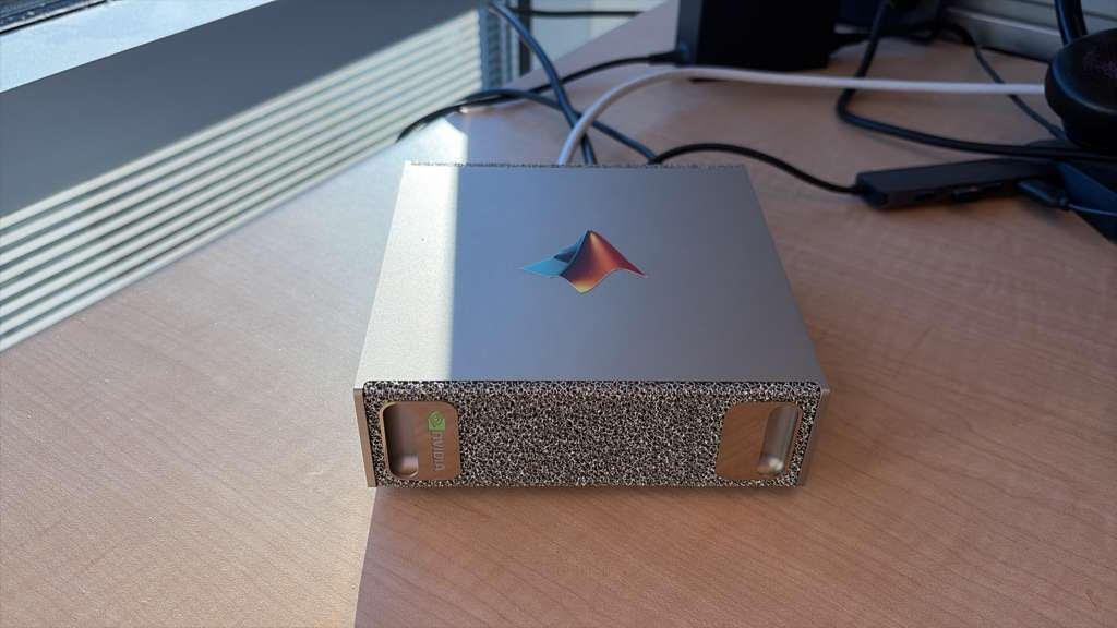
NVIDIA's DGX Spark is a small desktop machine that doesn't cost the earth. Indeed, several of us at MathWorks have one now although 'mine' (pictured above sporting a MATLAB sticker) is actually shared with a few other people and lives on a desk in Natick, USA while I'm in the UK.
The DGX Spark has 128GB of memory available to the GPU which means that I can run a MUCH larger language model. So, I installed a 120 Billion parameter model on it: gpt-oss:120b. More than an order of magnitude bigger than any local model I had played with before.
The next step was to connect to it from MATLAB running on my laptop.
The result is a *completely private* MATLAB + AI workflow that several of us have been playing with.
In my latest article, I show you how to set everything up: The LLM running on the DGX Spark connected to MATLAB running on my MacBook Pro. https://blogs.mathworks.com/matlab/2026/01/05/running-large-language-models-on-the-nvidia-dgx-spark-and-connecting-to-them-in-matlab/
This article describes how to prototype a physics simulation in HTML5 with Claude desktop App and then to replicate and deploy this product in MATLAB as an interactive GUI script. It also demonstrates how to use Claude Chrome Extension to operate MATLAB Online and App Designer to build bonafide MATLAB Apps with AI online.
Setup
My setup is a MacBook with Claude App with MATLAB (v2025a), MATLAB MCP Core Serve,r and various cloud related MCP tools. This setup allows Claude App to operate MATLAB locally and to manage files. I also have Claude Chrome Extension. A new feature in Claude App is a coding tab connected to Claude code file management locally.
Building HTML5 and MATLAB interactive applications with Claude App
In exploring the new Claude App tab, Claude suggested a variety of projects and I elected to build an HTML5 physics simulation. The Claude App interface has built-in rendering for artifacts including .html, .jsx, .svg, .md, .mermaid, and .pdf so an HTML5 interactive app artifact produced appears active right in Claude App. That’s fun and I had the thought that HTML5 would be a speedy way to prototype MATLAB code without evenconnecting to MATLAB.
I chose to simulateof a double pendulum, well known to exhibit chaotic motion, a simulation that students and instructors of physics might use to easily explore chaos interactively. I knew the project would entail numerical integration so was not entirely trivial in HTML5, and would later be relatively easy and more precise in MATLAB using ode45.
One thing led to another and shortly I had built a prototype HTML5 interactive app and then a MATLAB version and deployed it to my MATLAB Apps library. I didn’t write a line of code. Everything I describe and exhibit here was AI generated. It could have been hands-free. I can talk to Claude via Siri or via an interface Claude helped me build using MATLAB speech-to-text ( I have taught Claude to speak its responses back to me but that’s another story.)
A remarkable thing I learned is not just the AI’s ability to write HTML5 code in addition to MATLAB code, but its knowledge and intuition about app layout and user interactions. I played the role of an increasingly demanding user-experience tester, exercising and providing feedback on the interface, issuing prompts like “Add drag please” (Voila, a new drag slider with appropriately set limits and default value appears.) and “I want to be able to drag the pendulum masses, not just set angles via sliders, thank you.” Then “Convert this into a MATLAB code.”
I was essentially done in 45 minutes start to finish, added a last request, and went to bed. This morning I was just wondering and asked, “Any chance we can make this a MATLAB App?” and voila it was packaged and added to my Apps Library with an install file for others to use it. I will park these products on File Exchange for those who want to try out the Double Pendulum simulation. Later I realized this was not exactly what I had in mind
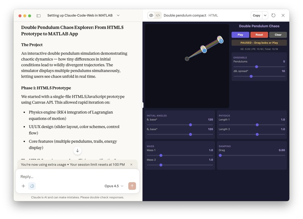
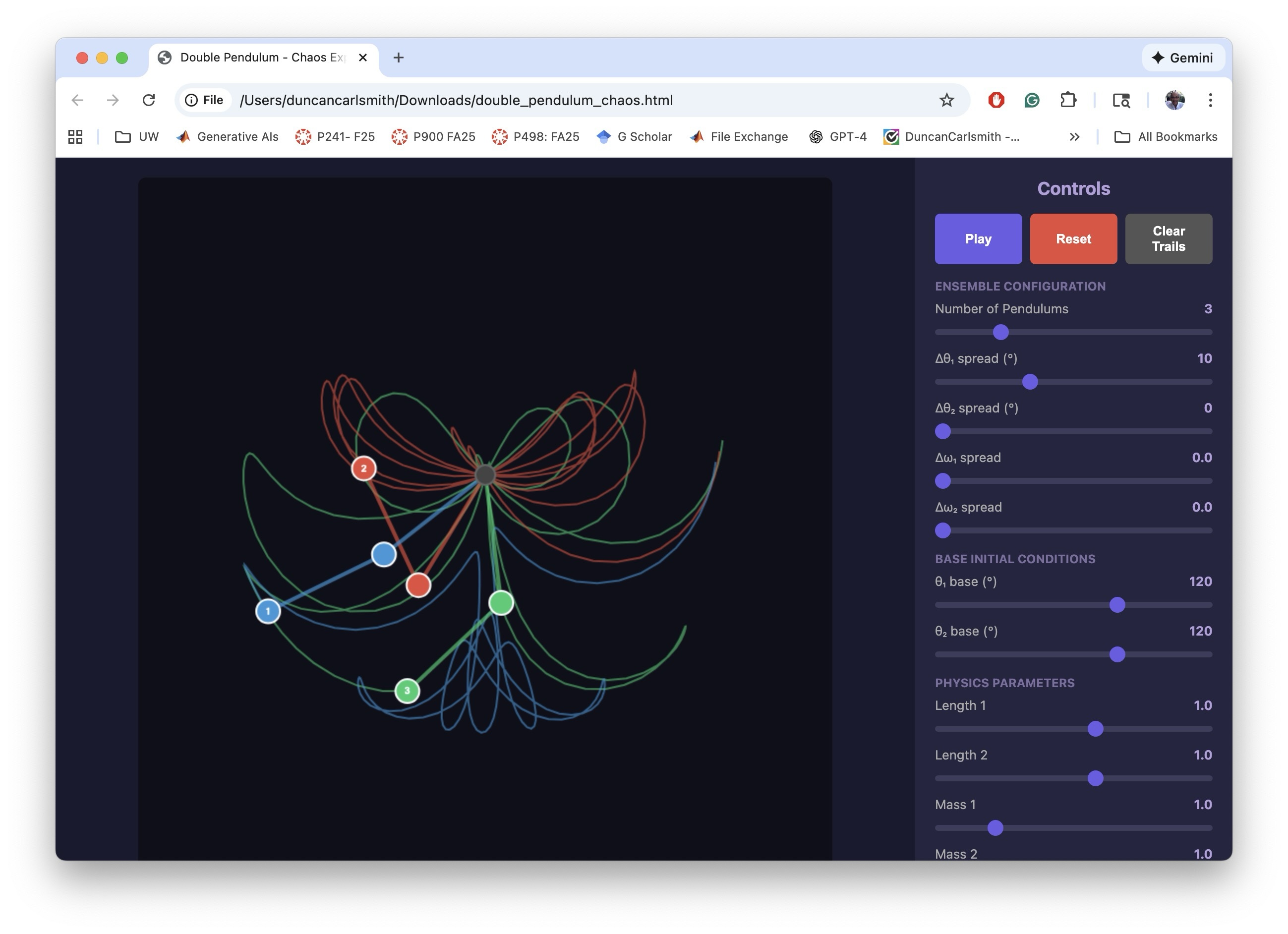
The screenshot below shows the Claude interface at the end of the process. The HTML5 product is fully operational in the artifacts pane on the right. One can select the number of simultaneous pendulums and ranges for initial conditions and click the play button right there in Claude App to observe how small perturbations result in divergence in the motions (chaos) for large pendulum angles, and the effect of damping.
The following image below show the HTML5 in a Chrome Browser window.
I making the MATLAB equivalent of the HTML5 app, I iterated a bit on the interactive features. The app has to trap user actions, consider possible sequences of choices, and be aware of timing. Success and satisfaction took several iteractions.
The screenshot below shows the final interactive MATLAB .m script running in MATLAB. The script creates a figure with interactive controls mirroring the HTML5 version. The DoublePendulumApp.mlappinstall file in the Files pane, created by Claude, copies the .m to the MATLAB/Apps folder and adds a button to the APPS Tab in the MATLAB tool strip.

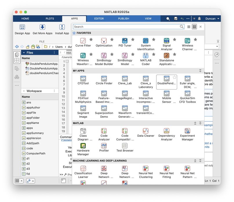
Below, you can see the MATLAB APP in my Apps Library.
To be clear, what was created in this process was not a true .mlapp binary file that would be created by MATLAB App Designer. In my setup, with MATLAB operating locally, Claude has no access to App Designer interactive windows via Puppeteer. It might be given access via some APPLE Script or other OS-specific trick but I’ve not pursued such options.
Claude Chrome Extension and App Designer online
To test if one could build actual Apps in the MATLAB sense with App Designer and Claude, I opened Claude Chrome Extension (beta) in Chrome in one tab and logged into MATLAB Online in another. Via the Chrome extension, Claude has access to the MATLAB Online IDE GUI and command line. I asked Claude to open App Designer and make a start on a prototype project. It can ferreted around in available MathWorks documentation, used MATLAB Online help vi the GUI I think, and performed some experiments to understand how to operate App Designer, and figured it out.
The screenshot below demonstrates a succesful first test of building an App Designer app from scratch. On the left is part of a Chrome window showing the Claude AI interface on the right hand side of a Chrome tab that is mostly off screen. On the right in the screenshot is MATLAB App Designer in a Chrome tab. A first button has been dragged on to the Design View frame in App Designer.

I only wanted to know if this workflow was possible, not build say the random quote generator Claude suggested. I have successfully operated MATLAB Online via Perplexity Comet Browser but not tried to operate APP Designer. Comet might be an alternate choice for this sort of task.
A word of caution. It is not clear to me that a Chrome Extension chat is available post facto through your regular Claude account, yet.
Appendix
This appendix is a summary generated by Claude of the development process and offers some additional details.
Double Pendulum Chaos Explorer: From HTML5 Prototype to MATLAB App
Author: Claude (Anthropic)
The Project
An interactive double pendulum simulation demonstrating chaotic dynamics — how tiny differences in initial conditions lead to wildly divergent trajectories. The simulator displays multiple pendulums simultaneously, letting users see chaos unfold in real time.
Phase 1: HTML5 Prototype
We started with a single-file HTML5/JavaScript prototype using Canvas API. This allowed rapid iteration on:
• Physics engine (RK4 integration of Lagrangian equations of motion)
• UI/UX design (slider layout, color schemes, control flow)
• Core features (multiple pendulums, trails, energy display)
The HTML5 version served as a "living specification" — we could test ideas in the browser instantly before committing to MATLAB implementation.
Phase 2: MATLAB GUI Development
Converting to MATLAB revealed platform-specific challenges:
Function name conflicts — Internal function names like updateFrame collided with Robotics Toolbox. Solution: prefix all functions with dp (e.g., dpUpdateFrame).
Timer-based animation — MATLAB's timer callbacks require careful state management via fig.UserData.
Robustness — Users can interact with sliders mid-animation. Every callback needed try-catch protection and proper pause/reinitialize logic.
Graphics cleanup — Changing pendulum count mid-run left orphaned graphics objects. Fixed with explicit cla() and handle deletion.
Key insight: The HTML5 prototype's logic translated almost directly, but MATLAB's callback architecture demanded defensive programming throughout.
Phase 3: MATLAB App Packaging
The final .m file was packaged as an installable MATLAB App using matlab.apputil.package(). This creates a .mlappinstall file that:
• Installs with a double-click
• Appears in MATLAB's APPS toolbar
• Can be shared with colleagues who have MATLAB
Files Produced
double_pendulum_chaos.html — Standalone browser version
doublePendulumChaosExplorer.m — MATLAB source code
DoublePendulumApp.mlappinstall — Shareable MATLAB App installer
Takeaways
1. Prototype in HTML5 — Fast iteration, instant feedback, platform-independent testing
2. Port to MATLAB — Same physics, different UI paradigm; expect callback/state management work
3. Package as App — One command turns a .m file into a distributable app
The whole process — from first HTML5 sketch to installed MATLAB App — demonstrates how rapid prototyping in the browser can accelerate development of production tools in specialized environments like MATLAB.
Introduction
This article describes how I have used MATLAB, MCP, and other tools to enable AI desktop apps to communicate with and share information between multiple AIs in performing research and code development. I describe how Claude desktop app (for example) can orchestrate AI-related setups of itself and other AI dektop apps using system calls through MATLAB, access multiple local and cloud AIs to develop and test code, and share with and evaluate results from multiple AIs. If you have been copy-pasting between MATLAB and an AI application or browser page, you may find this helpful.
Warning
When connected to MATLAB App via MCP, an AI desktop application acquires MATLAB App's command line privileges, possibly full system privileges. Be careful what commands you approve.
Setup
Experiments with Claude code and MATLAB MCP Core Server describes how to link Claude App via MCP to a local MATLAB to create MATLAB scripts in your file system, operate MATLAB App to test them, collect errors sent to standard output, view created files, and iterate. Other AI apps can similarly configured as described here.
My setup is an APPLE M1 MacBook with MATLAB v2025a and ollama along with MATLAB MCP Core Server, ollama MCP, filesystem MCP, fetch MCP to access web pages, and puppeteer MCP to navigate and operate webpages like MATLAB Online. I have similarly Claude App, Perplexity App (which requires the PerplexityXPC helper for MCP since it's sandboxed as a Mac App Store app), and LM Studio App. As of this writing, ChatGPT App support for MCP connectors is currently in beta and possibly available to Pro users if setup enabled via a web browser. It is not described here.
The available MCP commands are:
filesystem MCP `read_text_file`, `read_media_file`, `write_file`, `edit_file`, `list_directory`, `search_files`, `get_file_info`, etc.
matlab MCP `evaluate_matlab_code`, `run_matlab_file`, `run_matlab_test_file`, `check_matlab_code`, `detect_matlab_toolboxes`
fetch MCP ‘fetch_html`, `fetch_markdown`, `fetch_txt`, `fetch_json` | Your Mac |
puppeteer MCP `puppeteer_navigate`, `puppeteer_screenshot`, `puppeteer_click`, `puppeteer_fill`, `puppeteer_evaluate`, etc.
ollama MCP ‘ollama_list’, ‘ollama_show’, ’ollama_pull’, ’ollama_push’, ’ollana_copy’, ’ ollama-create’, ’ollama_copy’, ’ollama_delete’, ’ollama_ps’, ’ollama_chat’, ’ollama_web_search’, ’ollama_web_fetch’
Claude App (for example) can help you find, download, install, and configure MCP services for itself and for other Apps. Claude App requires for this setup a json configuration file like
{
"mcpServers": {
"ollama": {
"command": "npx",
"args": ["-y", "ollama-mcp"],
"env": {
"OLLAMA_HOST": "http://localhost:11434"
}
},
"filesystem": {
"command": "npx",
"args": [
"-y",
"@modelcontextprotocol/server-filesystem",
"/Users/duncancarlsmith/Documents/MATLAB"
]
},
"matlab": {
"command": "/Users/duncancarlsmith/Developer/mcp-servers/matlab-mcp-core-server",
"args": ["--matlab-root", "/Applications/MATLAB_R2025a.app"]
},
"fetch": {
"command": "npx",
"args": ["-y", "mcp-fetch-server"]
},
"puppeteer": {
"command": "npx",
"args": ["-y", "@modelcontextprotocol/server-puppeteer"]
}
}
}
Various options for these services are available through Claude App’s Settings=>Connectors. If you first install and set up the MATLAB MCP with Claude App, then Claude can find and edit its own json file using MATLAB and help you (after quitting and restarting) to complete the installations of all of the other tools. I highly recommend using Claude App as a command post for installations although other desktop apps like Perplexity may serve equally well.
Perplexity App is manually configured using Settings=>Connectors and adding server names and commands as above. Perplexity XPC is included with the Perplexity App download . When you create connectors with Perplexity App, you are prompted to install Perplexity XPC to allow Perplexity App to spawn proceses outside its container. LM Studio is manually configured via its righthand sidebar terminal icon by selecting Install-> Edit mcp.json. The json is like Claude’s. Claude can tell/remind you exactly what to insert there.
One gotcha in this setup concerns the Ollama MCP server. Apparently the default json format setting fails and one must tell the AIs to use “markdown” when commuicating with it. This instruction can be made session by session but I have made it a permanent preference in Claude App by clicking my initials in the lower left of Claude App, selecting settings, and under “What preferences should claude consider in responses,” adding “When using ollama MCP tools (ollama_chat, ollama_generate), always set format="markdown" - the default json format returns empty responses.”
LM Studio by default points at an Open.ai API. Claude can tell you how to download a model, point LM Studio at a local Ollama model and set up LM Studio App with MCP. Be aware that the default context setting in LM Studio is too small. Be sure to max out the context slider for your selected model or you will experience an AI with a very short term memory and context overload failures. When running MATLAB, LM Studio will ask for a project directory. Under presets you can enter something like “When using MATLAB tools, always use /Users/duncancarlsmith/Documents/MATLAB as the project_path unless the user specifies otherwise.” and attach that to the context in any new chat. An alternate ollama desktop application is Ollama from ollama.com which can run large models in the cloud. I encountered some constraints with Ollama App so focus on LM Studio.
I have installed Large Language Models (LLMs) with MATLAB using the recommended Add-on Browser. I had Claude configure and test it. This package helps MATLAB communicate with external AIs via API and also with my native ollama. See the package information. To use it, one must define tools with MATLAB code. A tool is a function with a description that tells an LLM what the function does, what parameters it takes, and when to call it. FYI, Claude discovered my small ollama default model had not been trained to support tool and hallucinated a numerical calculaton rather than using a tool we set up to perform such a calculation with MATLAB with machine precision. Claude suggested and then orchestrated the download of the 7.1 GB model mistral-nemo model which supports tool calling so if using you are going to use tools be sure to use a tool aware model.
To interact with Ollama, Claude can use the MATLAB MCP server to execute MATLAB commands to use ollamaChat() from the LLMs-with-MATLAB package like “chat = ollamaChat("mistral-nemo");response = generate(chat, "Your question here”);” The ollamaChat function creates an object that communicates with Ollama's HTTP API running on localhost:11434. The generate function sends the prompt and returns the text response. Claude can also communicate with Ollama using the Ollama MCP server. Similarly, one can ask Claude to create tools for other AIs.
The tool capability allows one to define and suggest MATLAB functions that the Ollama model can request to use to, for example, to make exact numerical calculations in guiding its response. I have also the MATLAB Add-on MATLAB MCP HTTP Client which allows MATLAB to connect with cloud MCP servers. With this I can, for example, connect to an external MCP service to get JPL-quality (SPICE generated) ephemeris predictions for solar system objects and, say, plot Earth’s location in solar system barycentric coordinates and observe the deviations from a Keplerian orbit due of lunar and other gravitational interactions.
To connect with an external AI API such as openAI or Perplexity, you need an account and API key and this key must be set as an environmental variable in MATLAB. Claude can remind you how to create the environmental variable by hand or how you can place your key in a file and have Claude find and extract the key and define the environmental variable without you supplying it explicitly to Claude.
It should be pointed out that conversations and information are NOT shared between Desktop apps. For example, if I use Claude App to, via MATLAB, make an API transaction with ChatGPT or Perplexity in the cloud, the corresponding ChatGPT App or Perplexity App has no access the the transaction, not even to a log file indicating it occured. There may be various OS dependent tricks to enable communication between AI desktop apps (e.g. AppleScript/AppleEvents copy and paste) but I have not explored such options.
AI<->MATLAB Communication
WIth this setup, I can use any of the three desktop AI apps to create and execute a MATLAB script or to ask any supported LLM to do this. Only runtime standard output text like error messages generated by MATLAB are fed back via MCP. Too evaluate the results of a script during debugging and after successful execution, an AI requires more information.
Perplexity App can “see and understand” binary graphical output files (presented as inputs to the models like other data) without human intervention via screen sharing, obviating the need to save or paste figures. Perplexity and Claude can both “see” graphical output files dragged and dropped manually into their prompt interface. With MacOS, I can use Shift-Command-5 to capture a window or screen selection and paste it into the input field in either App. Can this exchange of information be accomplished programmatically? Yes, using MCP file services.
To test what binary image file formats are supported by Claude with the file server connection, I asked Claude to use MATLAB commands to make and convert a figure to JPEG, PNG, GIF, BMP, TIFF, and WebP and found the filesytem: read_media_file command of the Claude file server connection supported the first three. The file server MCP transmits the file using JSON and base64 text strings. A 64-bit encoding adds an additonal ~30 percent to a bitmap format and there is overhead. A total tranmission limit of 1MB is imposed by Anthropic so the maximum bitmap file size appears to be about 500 KB. If your output graphic file is larger, you may ask Claude to use MATLAB to compress it before reading it via the file service.
BTW, interestingly, the drag and drop method of image file transfer does not have this 500 KB limit. I dragged and dropped an out of context (never shared in my interactions with Claude) 3.3 MB JPEG and received a glowing, detailed description of my cat.
So in in generating a MATLAB script via AI prompts, we can ask the AI to make sure MATLAB commands are included in the script that save every figure in a supported and possibly compressed bitmap format so the command post can fetch it. Claude, for example, can ‘see’ an an annotated plot and and accurately describe the axes labels, understand the legend, extract numbers in an annotation, and also derive approximate XY values of a plotted function. Note that Claude (given some tutoring and an example) can also learn to parse and find all of the figures saved as PNG inside a saved .mlx package and, BTW, create a .mlx from scratch. So an alternate path is to generate a Live Script or ask the AI to convert a .m script to Live Script using a MATLAB command and to save the executed .mlx. Another option is for the AI to ask MATLAB to loop over figures and execute for each issue a command like exportgraphics(fig, ‘figname.png', 'Resolution', 150); and then itself upload the files for processing.
With a sacrifiice of security, other options are available. With the APPLE OS, it is possible to approve matlab_mcp_core_server (and or your Claude App or Perplexity App) to access screen and audio recording. Then for example, Claude can ask MATLAB to issue a system command system('screencapture -x file.png') to capture the entire screen or java.awt.Robot().createScreenCapture() to capture a screen window. I have demonstrated with Claude App capturing a screenshot showing MATLAB App and figures, and, for fun, sending that via API to ChatGPT, and receiving back an analysis of the contents. (Sending the screenshot to Perplexity various ways via API failed for unknown reasons despite asking Perplexity for help.)
One might also try to execute a code like
robot = java.awt.Robot();
toolkit = java.awt.Toolkit.getDefaultToolkit();
screenSize = toolkit.getScreenSize();
rectangle = java.awt.Rectangle(0, 0, screenSize.width, screenSize.height);
bufferedImage = robot.createScreenCapture(rectangle);
% ... convert to MATLAB array and save with imwrite()
to capture and transmit a certain portion of your screen. Going down this path further, according to Claude, it is possible to create a MacOS virtual Desktop containing only say MATLAB, Claude, and Perplexity apps so a screen capture does not accidentally transmit a Mail or Messages window. Given accessiblity permission, one could capture windows by ID and stitch them together with a MATLAB command like composite = [matlab_img; claude_img; perplexity_img]; imwrite(composite, 'ai_workspace.png');
One must be careful an AI does not fake an analysis of an image based on context. Use a prompt preface like ‘Based solely on this image,… .” Note that AI image analysis is useful if you want suggestions for how to improve a figure by say moving a legend location from some default ‘best location’ to another location where it doesn’t hide something important.
What about communicating exact numerical results from MATLAB to an AI? A MATLAB .fig format file contains all of the exact data values used to create the figure. It turns out, Claude can receive a .fig through the manually-operated attach-file option in Claude App. Claude App of course sends received data to Anthropic and can parse the .fig format using python in its Docker container. In this way it can access the exact values behind plot data points and fitted curves and, for example, calculate a statistic describing agreement between a model curve and the data, assess outliers, and in principle suggest actions like smoothing or cleaning. Perplexity App’s manual attach-file handler does not permit upload of this format. There seem to be workarounds to 64-bit encode output files like .fig and transfer them to the host (Anthropic or Perplexity) but are there simpler ways to communicate results of the script execution? Yes.
Unless one has cleared variables during execution, all numerical and other results are contained in workspace variables in MATLAB’s memory. The values of these variables if saved can be accessed by an AI using MATLAB commands. The simplest way to ensure these values are available is to ask the AI that created and tested the script to include in the script itself a command like save('workspace.mat’) or to ask MATLAB to execute this command after executing the script. Then any AI connected to MATLAB can issue a request for variable values by issuing a MATLAB command like ‘data=load(‘workspace.mat’);fprintf(‘somevariablename’);and receive the response as text. An AI connected to MATLAB can also garner data embedded in a saved figure using MATLAB with a command like fig = openfig('MassPlots.fig', 'invisible'); h = findall(fig, 'Type', 'histogram'); data = h.Values .
Example work flow
The screenshot below illustrates a test with this setup. On the right is Perplexity App. I had first asked Perplexity to tell me about Compact Muon Solenoid (CMS) open data at CERN. The CERN server provides access to several data file types through a web interface. I decided to analyze the simplest such files, namely, Higgs boson decay candidate csv files containing the four-momentum vectors of four high energy leptons (two electrons and two muons) in select events recorded in the early years 2011 and 2012. (While the Higgs boson was discovered via its top-quark/W-boson loop-mediated decay to two photons, it can also decay to two Z bosons and each of these to a lepton+antilepton pair of any flavor.)

I asked Perplexity to create a new folder and write a MATLAB code to download those two files into the folder. Perplexity asked me to mouse over and copy the URLs of the download links on the appropriate page as these were hidden behind java applications, and voila. (As a test, I asked Claude in vague terms to find and download these files and it just figured it out without my manual intervention.) Next I asked Perplexity to “write and execute a MATLAB script to histogram the invariant mass of the electron pairs, of the muon pairs, and of the entire system of leptons, and to overlay fits of each dilepton mass distribution to a Lorentzian peak near the Z-boson mass (~90 GeV) plus a smooth background, save the script in the same folder, and run it.” It turns out that uncorrelated Z-boson pairs can be created by radiation from uncorrelated processes, that virtual Z bosons and photons with the “wrong” mass can be created, so one does not expect to necessary see a prominence in the 4-lepton invariant mass at the Higgs mass. For this reason I did not ask for a fit to the 4-lepton mass distribution. I did provide the starting estimated value for the location of the peak based on my experience of such nonlinear fits going off the rails.
After approving a few fixes of minor errors, voila. Sweet. In the middle of the screen shot are MATLAB App and the figure created. The format of the figure was all invented by the AI. On the left is Claude App’s analysis of the data, extracted from the manually uploaded figure in .fig format. The prompt was “Extract the histogram and fit values bin by bin an calculate the chisq per degree of freedom using the data in that .fig upload” .
I manually saved the workspace using the MATLAB Command line ( I could have asked Claude to do that) and I issued to Claude App the prompt “OK, I just saved workspace.mat in MATLAB/CMS. List the contents and the fit results.” Below is an image of the response of Claude analyzing the workspace .mat file.

I then asked Claude to ask my local Ollama model for a 2nd opinion with the prompt “I want you to ask mistral-nemo for a 2nd opinion on the results on its own, based on all it knows, and to ask it for information about related resources. ” Claude first formulated and sentthe following prompt to the local LLM: “I measured the Z boson in the dimuon channel and got: Mass = 92.46 GeV Width = 12.44 GeV. The PDG values are M_Z = 91.19 GeV and Gamma_Z = 2.50 GeV. Based on your knowledge of particle physics and detector effects, what do you think is going on with my measurement? What could cause the width to be 5x larger than the natural width?” It’s mention of the width discrepency inparticular indicated it knew more about the physics than it had divulged.
Claude used MATLAB to call the local Ollama's REST API to get mistral-nemo's opinion with the path MATLAB MCP → webwrite() → Ollama Server (localhost:11434) → mistral-nemo% calling Ollama's API from MATLAB with the pattern url = 'http://localhost:11434/api/generate';body = struct('model', 'mistral-nemo', 'prompt', 'Your question...', 'stream', false);response = webwrite(url, body, weboptions('MediaType', 'application/json'));
The received response was:
Your measured results for the Z boson mass and width differ significantly from the Particle Data Group (PDG) values. Here's a possible explanation for these discrepancies:
1. **Mass:**
The measured mass of 92.46 GeV is about 1.3 GeV higher than the PDG value of 91.19 GeV. This could be due to:
- **Detector calibration issues**: If your detector's energy scale is slightly miscalibrated, it could lead to an apparent shift in the measured mass.
- **Systematic effects**: Unaccounted-for systematic uncertainties might contribute to this difference.
- **New Physics**: While less likely, if new physics processes affect the Z boson, they could cause a resonant rise or other deviations from the expected behavior.
2. **Width:**
The measured width of 12.44 GeV is roughly five times larger than the natural width (Gamma_Z = 2.50 GeV). This significant difference is concerning and suggests potential issues:
- **Resonance tail**: If there's an unknown resonance near the Z boson mass, it could contribute to a large apparent width.
- **Misestimation of experimental resolution**: If you have underestimated your detector's energy resolution, it might result in a broader observed peak. The difference here seems quite large compared to typical experimental uncertainties (~1-2%).
- **Backgrounds and pile-up**: Higher backgrounds or pile-up events could artificially broaden the width.
- **Analysis method**: There might be an issue with your analysis method leading to a biased estimation of the Z boson width.
Given the discrepancy in both mass and width, it's crucial to perform thorough checks and validations:
- Review detector calibration data.
- Evaluate systematic uncertainties.
- Check for potential instrumental effects or electronic issues with the detector.
- Verify background models and consider alternative fitting methods or techniques like sideband subtraction.
- Re-evaluate your analysis pipeline to ensure no steps lead to biases in the measurements.
- Consult colleagues or experts to help identify possible causes of the discrepancy.
If these checks don't resolve the issue, it might warrant a cautionary note on potential new physics processes affecting the Z boson. However, without solid evidence and careful validation, it would be premature to claim such findings at this stage.
Claude then prompted the Ollama model with “I’m analyzing CMS H→ZZ→4ℓ data to measure Z boson properties. Can you recommend:1. Key papers I should read on Z boson measurements at the LHC 2. Standard analysis techniques for handling detector resolution 3. Any publicly available CMS or ATLAS open data resources 4. Software tools commonly used for this type of analysis” and received a long list of resources.
As Claude pointed out, the local Ollama model operates purely from memory and is subject to URL hallunciation so I asked Claude to check each of the many (too many to list here) URLs that Ollama provided. Claude has several options to accomplish such a task in my setup:
1. web_fetch (Anthropic tool)
2. fetch MCP server (installed on my Mac) commands fetch_html, fetch_markdown, fetch_text, fetch_jason.
3. puppeteer MCP server (installed on my Mac) which can navigate to a URL and take a screen shot and handle JavaScript-rendered pages.
4. web_search (Anthropic tool)
5. MATLAB web access tools including webread, websave, and shell commands
Claude first chose to test Ollama’s references using my installed fetch MCP server and found Mistral-nemo's URL accuracy to be: 5 valid: opendata.cern.ch, root.cern.ch, opendata.atlas.cern, pythia.org (concept, wrong URL), cms-sw.github.io; 6 invalid/hallucinated: atlas-open-data.org, pythia8.hep.yorku.ca, aida.hep.com, mc-code.eu/sherpa, www.cms.gov; 2 exist but WRONG CONTENT: arxiv URLs exist but are completely unrelated papers!
However, as Claude pointed out, use of one tool alone is subject to gotcha’s due to the variety of webpage content and deployment, robot rejection methods, and ability to check the content is valid if the URL is in fact reachable so a more detailed winnowing of the supplied resources ensued, combining results from using all tools.
Puppeteer
So what does the puppeteer server bring to the table? Puppeteer allows an app to access a website and exercise its interface. I used it with Claude App to explore and understand the interactive tools for creating an article submission on this website. Rather than create this submission, based on my own experience and Claude’s help, decided tht rather than have Claude build the submission interactively, it was easiest this time to create the submission in formatted .rtfd and paste that manually into the article submission field retaining all formating, and possibly use MATLAB to downsize the graphics a bit before insertion. WIth more experience, all this could be automated.
Like Perplexity Comet and the new Claude Chrome Extension, with puppeteer, your desktop AI App can presumably operate MATLAB Online but I’ve yet to explore that. If you do, let me know how it goes.
Conclusion
I hope this article encourages you to explore for yourself the use of AI apps connected to MATLAB, your operating system, and to cloud resources including other AIs. I am more and more astounded by AI capabilities. Having my “command post” suggest, write, test, and debug code, anwser my questions, and explore options was essential for me. I could ot have put this together unasisted. Appendix 1 (by Claude) delves deeper into the communications processes and may be helpful. Appendix 2 provides example AI-agent code generated by Claude. A much more extensive one was generated for interaction with Claude. To explore this further, ask Claude to just build and test such tools.
References
Appendix 1 Understanding the Architecture (Claude authored)
What is MCP?
Model Context Protocol (MCP) is an open standard developed by Anthropic that allows AI applications to connect to external tools through a standardized interface. To understand how it works, you need to know where each piece runs and how they communicate.
Where Claude Actually Runs
When you use Claude Desktop App, the AI model itself runs on Anthropic's cloud servers — not on your Mac. Your prompts travel over HTTPS to Anthropic, Claude processes them remotely, and responses return the same way. This raises an obvious question: how can a remote AI interact with your local MATLAB installation?
The Role of Claude Desktop App
Claude Desktop App is a native macOS application that serves two roles:
- Chat interface: The window where you type and read responses
- MCP client: A bridge that connects the remote Claude model to local tools
When you launch Claude Desktop, macOS creates a process for it. The app then reads its configuration file (~/Library/Application Support/Claude/claude_desktop_config.json) and spawns a child process for each configured MCP server. These aren't network servers — they're lightweight programs that communicate with Claude Desktop through Unix stdio pipes (the same mechanism shell pipelines use).
┌─────────────────────────────────────────────────────────────────┐
│ Your Mac │
│ │
│ Claude Desktop App (parent process) │
│ │ │
│ ├──[stdio pipe]──► node ollama-mcp (child process) │
│ ├──[stdio pipe]──► node server-filesystem (child) │
│ ├──[stdio pipe]──► matlab-mcp-core-server (child) │
│ ├──[stdio pipe]──► node mcp-fetch-server (child) │
│ └──[stdio pipe]──► node server-puppeteer (child) │
│ │
└─────────────────────────────────────────────────────────────────┘
When you quit Claude Desktop, all these child processes terminate with it.
The Request/Response Flow
Here's what happens when you ask Claude to run MATLAB code:
- You type your request in Claude Desktop App
- Claude Desktop → Anthropic (HTTPS): Your message travels to Anthropic's servers, along with a list of available tools from your MCP servers
- Claude processes (on Anthropic's servers): The model decides to use the evaluate_matlab_code tool and generates a tool-use request
- Anthropic → Claude Desktop (HTTPS): The response arrives containing the tool request
- Claude Desktop → MCP Server (stdio pipe): The app writes a JSON-RPC message to the MATLAB MCP server's stdin
- MCP Server executes: The server runs your code in MATLAB and captures the output
- MCP Server → Claude Desktop (stdio pipe): Results written to stdout
- Claude Desktop → Anthropic (HTTPS): Tool results sent back to Claude
- Claude formulates response (on Anthropic's servers)
- Anthropic → Claude Desktop → You: Final response displayed
The Claude model never directly touches your machine. It can only "see" what MCP servers return, and it can only "do" things by requesting tool calls that your local app executes on its behalf.
MCP Servers vs. Backend Services
It's important to distinguish MCP servers from the services they connect to:
Component
What It Is
Lifecycle
Ollama MCP server
A Node.js process that translates MCP requests into Ollama API calls
Spawned by Claude Desktop, dies when app quits
Ollama server
The actual LLM runtime serving models like mistral-nemo
Runs independently (started manually or via launchd)
MATLAB MCP server
A process that translates MCP requests into MATLAB Engine commands
Spawned by Claude Desktop
MATLAB
The full MATLAB application
Runs independently; MCP server connects to it
If the Ollama server isn't running, the Ollama MCP server has nothing to talk to — its commands will fail. Similarly, the MATLAB MCP server needs MATLAB to be running (or may launch it, depending on implementation).
What About Other AI Apps?
If you run both Claude Desktop and Perplexity App with MCP configurations, each app spawns its own set of MCP server processes:
Claude Desktop (PID 1001) Perplexity App (PID 2001)
│ │
├── ollama-mcp (PID 1002) ├── ollama-mcp (PID 2002)
├── server-filesystem (PID 1003) ├── server-filesystem (PID 2003)
└── matlab-mcp-server (PID 1004) └── matlab-mcp-server (PID 2004)
│ │
│ HTTP to same endpoints │
└──────────────►◄──────────────────────┘
│
┌──────────┴──────────┐
│ Shared Services │
│ • Ollama Server │
│ • MATLAB Engine │
└─────────────────────┘
Key points:
- No cross-talk: Claude Desktop cannot communicate with Perplexity's MCP servers (or vice versa). Each app only talks to its own children via stdio pipes.
- Shared backends: Both apps' MCP servers can make requests to the same Ollama server or MATLAB instance — they're just independent clients of those services.
- No app launching: Claude cannot launch, control, or send commands to Perplexity App. They are peer applications, not parent-child.
How Claude "Talks To" Perplexity
When I say Claude can query Perplexity, I mean Claude calls Perplexity's cloud API — not Perplexity App. The path looks like this:
Claude model (Anthropic servers)
│
│ requests tool use
▼
Claude Desktop App
│
│ stdio pipe
▼
MATLAB MCP Server
│
│ MATLAB Engine API
▼
MATLAB running webwrite() or perplexityAgent()
│
│ HTTPS
▼
api.perplexity.ai (Perplexity's cloud)
Perplexity App isn't involved at all. The same applies to OpenAI, Anthropic's own API (for nested calls), or any other service with an HTTP API.
One App to Rule Them All?
Claude Desktop doesn't control other apps, but it can:
- Orchestrate local tools via MCP servers it spawns and controls
- Call any cloud API (Perplexity, OpenAI, custom services) via HTTP through fetch MCP or MATLAB
- Share backend services (Ollama, MATLAB) with other apps that happen to use them
- Coordinate multi-AI workflows by sending prompts to local models (via Ollama) and cloud APIs, then synthesizing their responses
The "ruling" is really about Claude serving as a command post that can dispatch requests to many AI backends and tools, not about controlling other desktop applications.
Appendix 2 Example AI agent (Claude authored)
The following is an example of Claude-generated code generated for an AI agent to handle requests to access Perplexity. It receives the users prompt, if needed, discovers the users Perplexity API key hidden in a local text file, posts a message to Perplexity API, and then receives and returns the response.
function response = perplexityAgent(prompt)
%PERPLEXITYAGENT Query Perplexity AI using their Sonar API
% response = perplexityAgent(prompt)
%
% Requires: PERPLEXITY_API_KEY environment variable
% Get your key at: https://www.perplexity.ai/settings/api
apiKey = getenv('PERPLEXITY_API_KEY');
if isempty(apiKey)
% Try to load from file
keyFile = fullfile(userpath, 'PERPLEXITY_API_KEY.txt');
if isfile(keyFile)
fid = fopen(keyFile, 'r');
raw = fread(fid, '*char')';
fclose(fid);
match = regexp(raw, 'pplx-[a-]+', 'match');
if ~isempty(match)
apiKey = match{1};
setenv('PERPLEXITY_API_KEY', apiKey);
end
end
end
if isempty(apiKey)
error('PERPLEXITY_API_KEY not set. Get one at perplexity.ai/settings/api');
end
url = 'https://api.perplexity.ai/chat/completions';
% Build request
data = struct();
data.model = 'sonar';
msg = struct('role', 'user', 'content', prompt);
data.messages = {msg};
jsonStr = jsonencode(data);
% Use curl for reliability
curlCmd = sprintf(['curl -s -X POST "%s" ' ...
'-H "Authorization: Bearer %s" ' ...
'-H "Content-Type: application/json" ' ...
'-d ''%s'''], url, apiKey, jsonStr);
[status, result] = system(curlCmd);
if status == 0 && ~isempty(result)
resp = jsondecode(result);
if isfield(resp, 'choices')
response = resp.choices(1).message.content;
elseif isfield(resp, 'error')
response = sprintf('API Error: %s', resp.error.message);
else
response = result;
end
else
response = sprintf('Request failed with status %d', status);
end
end
Introduction
Experiments with Claude code and MATLAB MCP Core Server describes how to link Claude App to a local MATLAB such that Claude can read and write scripts on your file system, operate MATLAB App to test them, collect errors, and iterate, obviating the need for copy-pasting between Claude App and MATLAB. Here I describe how one can achieve essentially the same functionality with Perplexity App, conveniently provide graphical results to Perplexity via screen sharing rather than by saving figures to files, and simultaneously run both Perplexity and Claude Apps thusly connected.
Setup
To allow Perplexity App to read and write files, go to Perplexity Settings-> Connectors-> Browse Connectors and select Filesystem. To add an installed MATLAB MCP, go to Perplexity Settings-> Connectors-> Add Connector. Here, under the Simple tab, you can add any server name, say MATLAB MCP, and a command like /Users/duncancarlsmith/Developer/mcp-servers/matlab-mcp-core-server --matlab-root /Applications/MATLAB_R2025a.app pointing to your MATLAB App. Then, under advanced, add JSON configuration code that points to the location of the matlab-mcp=cos=server such as
{
"args" : [
"--matlab-root",
"/Applications/MATLAB_R2025a.app"
],
"command" : "/Users/duncancarlsmith/Developer/mcp-servers/matlab-mcp-core-server",
"env" : {
},
"useBuiltInNode" : true
}
I append a Perplexity-generated summary of installation steps and gotcha’s.
Example test
In the screenshot below, you see the Perplexity App on the left after it created a test folder and a simple MATLAB test script to plot a function. It has recently changed the value of a code parameter from 2 to 3. The script appears in the MATLAB window along with a figure it produced when run. At the lower right appears Claude App. It has just changed that value to 4, thank you.
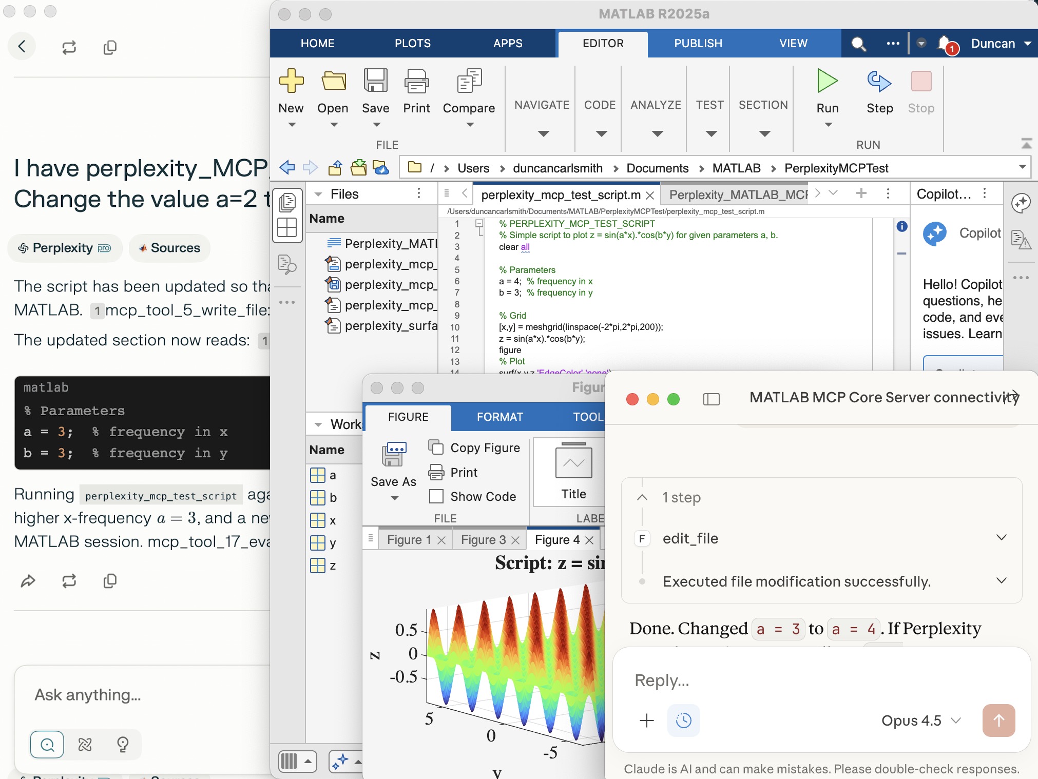
Note that Perplexity App’s file system access, like Claude App’s access, is limited to a folder of your choice, but both can issue system commands through MATLAB, so they inherit MATLAB’s privileges. Access can be restricted on a Mac by denying full disk access under Sytem Settings->Privacy and Security->Full Disk Access but that may be insufficient protection. Be careful. Also, when issuing a command to the MCP Server, both require you to review and approve any operation by default and allow you to override that behavior.
Screen sharing with Perplexity
While Perplexity and Claude Apps do not “see” figures and other non-standard output via the MCP server unless saved to files the can access through its file server, Perplexity can in fact see the graphical results of a code and more through screen sharing, as demonstrated in the screenshot below of Perplexity App. At the bottom, below the Perplexity input form field, just to the left of the microphone, is a button enabling Perplexity to accept screen sharing from a selection of windows. I selected the MATLAB App window and the MATLAB Figure window and then asked Perplexity to describe the contents. Images of these wondows appear in the response as well as descriptions of the images. Sweet! No longer must I attempt to provide feedback by attempting to describe such results myself in words.
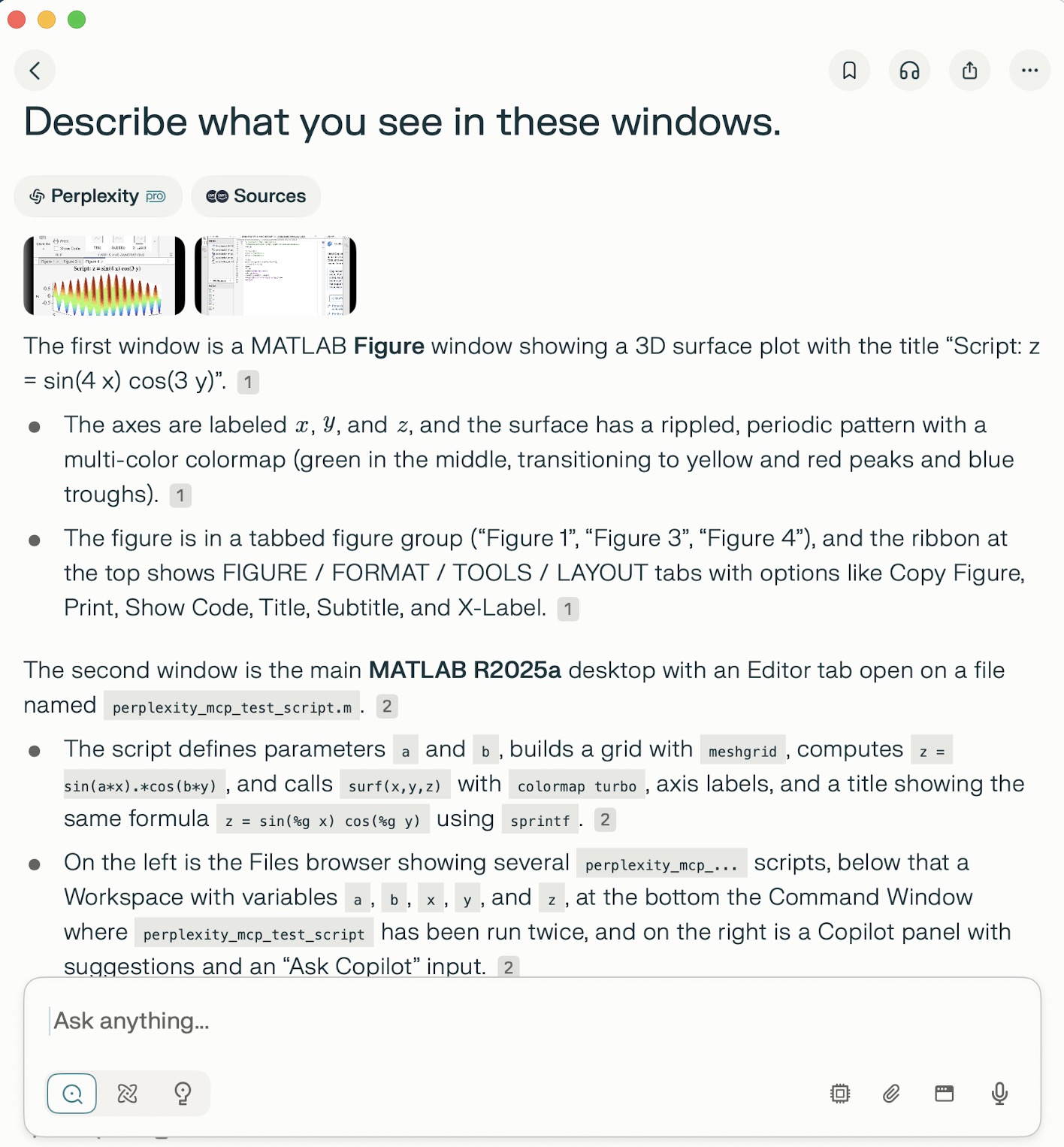
Appendix
(by Perplexity App)
Perplexity + MATLAB MCP Core Server Setup (macOS, R2025a)
1. Install and locate MATLAB
- Ensure MATLAB R2025a (or your chosen version) is installed under /Applications (e.g., /Applications/MATLAB_R2025a.app).
- From Terminal, verify MATLAB works:
"/Applications/MATLAB_R2025a.app/bin/matlab" -batch "ver"
This should list MATLAB and toolboxes without errors.
2. Fix PATH and shell alias for matlab
- Confirm the shell resolves the correct matlab:
which matlab
- If it is missing or points to an old version (e.g., R2022b), adjust:
export PATH="/Applications/MATLAB_R2025a.app/bin:$PATH"
which matlab
- Clear any stale alias or function:
type matlab
unalias matlab 2>/dev/null
unset -f matlab 2>/dev/null
which matlab
matlab -batch "ver"
Now matlab should invoke R2025a.
3. Place the MATLAB MCP Core Server binary
- Put the matlab-mcp-core-server binary in a convenient folder, e.g.:
/Users/duncancarlsmith/Developer/mcp-servers/matlab-mcp-core-server
- Make it executable:
cd /Users/duncancarlsmith/Developer/mcp-servers
chmod +x matlab-mcp-core-server
4. (Optional sanity check) Run the core server manually
- In Terminal, start the server once to confirm it can see MATLAB:
cd /Users/duncancarlsmith/Developer/mcp-servers
mkdir -p "$HOME/Claude-MATLAB-work"
./matlab-mcp-core-server \
--matlab-root="/Applications/MATLAB_R2025a.app" \
--initial-working-folder="$HOME/Claude-MATLAB-work"
- You should see INFO logs ending with:
"MATLAB MCP Core Server application startup complete".
- This process is not required long term once Perplexity is configured to launch the server itself.
5. Configure the MATLAB MCP connector in Perplexity (Mac app)
- Open Perplexity.
- Go to Settings → Connectors → Add Connector (or edit existing).
- Simple tab:
- Server command:
/Users/duncancarlsmith/Developer/mcp-servers/matlab-mcp-core-server --matlab-root /Applications/MATLAB_R2025a.app
- Advanced tab for the same connector:
{
"args": [
"--matlab-root",
"/Applications/MATLAB_R2025a.app"
],
"command": "/Users/duncancarlsmith/Developer/mcp-servers/matlab-mcp-core-server",
"env": {
},
"useBuiltInNode": true
}
- Save and ensure the connector shows as enabled.
6. Configure the filesystem MCP connector for MATLAB files
- Install the filesystem MCP server (one-time):
npx -y @modelcontextprotocol/server-filesystem /Users/duncancarlsmith/Documents/MATLAB
- In Perplexity Settings → Connectors → Add Connector:
- Name: filesystem (or similar).
- Server command:
npx -y @modelcontextprotocol/server-filesystem /Users/duncancarlsmith/Documents/MATLAB
- This allows Perplexity to list, create, and edit files directly under ~/Documents/MATLAB.
7. Test connectivity from Perplexity
- Start a new thread in Perplexity, with both the MATLAB connector and filesystem connector enabled.
- Verify MATLAB access by listing toolboxes or running a simple command via MCP:
- For example, list the contents of ~/Documents/MATLAB.
- Create a test folder (e.g., PerplexityMCPTest) using MATLAB or filesystem tools and confirm it appears.
8. Create and run a simple MATLAB script via Perplexity
- Using the filesystem connector, create a script in PerplexityMCPTest, e.g. perplexity_mcp_test_script.m:
% PERPLEXITY_MCP_TEST_SCRIPT
% Simple script to plot z = sin(a*x).*cos(b*y) for given parameters a, b.
clear all
% Parameters
a = 2; % frequency in x
b = 3; % frequency in y
% Grid
[x,y] = meshgrid(linspace(-2*pi,2*pi,200));
z = sin(a*x).*cos(b*y);
figure
% Plot
surf(x,y,z,'EdgeColor','none');
colormap turbo;
xlabel('x'); ylabel('y'); zlabel('z');
title(sprintf('Script: z = sin(%g x) cos(%g y)',a,b));
axis tight;
- From Perplexity, call MATLAB via the MCP server to run:
cd('PerplexityMCPTest'); perplexity_mcp_test_script
- In the local MATLAB desktop, a figure window will appear with the plotted surface.
9. Notes on behavior
- Perplexity interacts with MATLAB through the MCP Core Server and does not see the MATLAB GUI or figures; only text output/errors are visible to Perplexity.
- A brief extra MATLAB window may appear and disappear when the core server starts or manages its own MATLAB session; this is expected and separate from your own interactive MATLAB instance.
- File creation and editing from Perplexity occur via the filesystem MCP server and are limited to the configured root (here, ~/Documents/MATLAB).