Results for
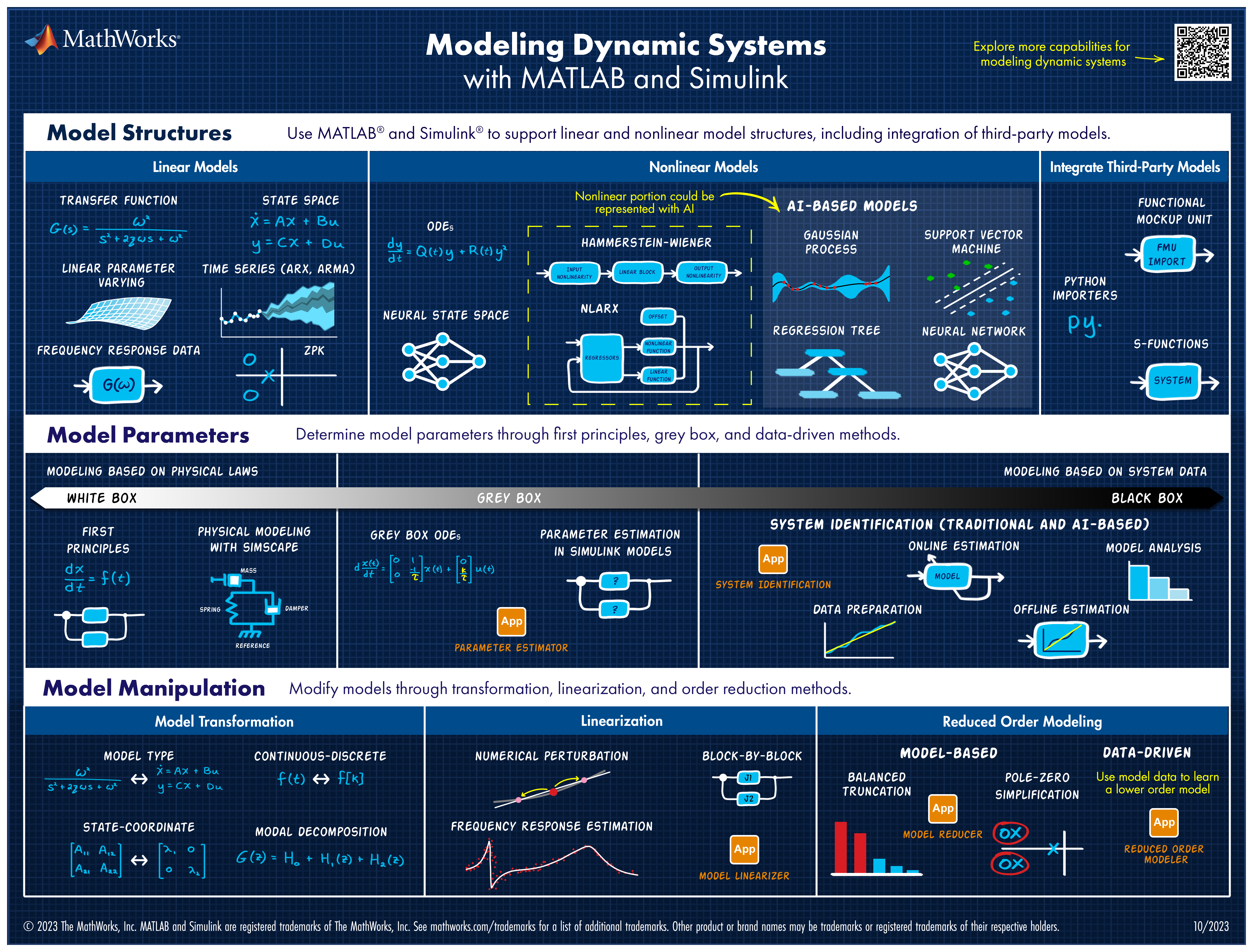
Explore all the capabilities for Modeling Dynamic Systems while keeping them handy with this Cheat Sheet - Download Now.
Hi,
I'm trying to install R2023b silently on Windows 10 Enterprise 22H2. The process starts but fails 10% into everything.
End of the file C:\tempmatlab\R2023b\installer_input.txt
(Dec 20, 2023 08:43:48) Session key: 5955da33-7f96-454a-b24a-aa1914758a09
(Dec 20, 2023 08:43:49) Product Files Folder: C:\tempmatlab\R2023b\archives
(Dec 20, 2023 08:43:52) License Agreement validation is successful.
(Dec 20, 2023 08:43:52) FIK validation is successful.
(Dec 20, 2023 08:43:52) License File validation is successful.
(Dec 20, 2023 08:43:52) Folder validation is successful.
(Dec 20, 2023 08:43:52) Product selection validation is successful.
(Dec 20, 2023 08:43:52) Confirm Selections
(Dec 20, 2023 08:43:52) Destination
(Dec 20, 2023 08:43:52) C:\Program Files\MATLAB\R2023b
(Dec 20, 2023 08:43:52) Products
(Dec 20, 2023 08:43:52) 113 of 113 products
(Dec 20, 2023 08:43:52) 23.74 GB required
(Dec 20, 2023 08:44:47) 1%
(Dec 20, 2023 08:45:09) 2%
(Dec 20, 2023 08:46:25) 3%
(Dec 20, 2023 08:46:40) 4%
(Dec 20, 2023 08:47:12) 5%
(Dec 20, 2023 08:47:20) 10%
(Dec 20, 2023 08:47:48) Exiting with status -2
(Dec 20, 2023 08:47:48) End - Unsuccessful
Both a FIK & license.dat are accessible during the install. There is 80GB of free disk space as well. No one is logged in to Windows when the install is performed. What does status -2 mean?
Thnaks!
I have encountered a problem. I want to study the direction of PHEVP2 configuration energy control strategy, but the whole vehicle model has stumped me. I don't know how to proceed, and every time I run, an error message will be reported. I don't understand where the problem lies?
Никак не получается создать новый ThinkHTTP так как пишет что URL?АДРЕСС СТРАНИЦЕ НЕ ДЕЙСТВИТЕЛЬНЫЙ
Here's the English translation. "I can't create a new ThinkHTTP because it says that the URL is not valid"
I'm going to customize the example of the MATLAB px4 hitl simulation and apply it to our current plane called SkysurferX8. I've calculated the aerodynamic factor and put it all in, but there's a problem. I wonder which code part of the example should be modified for trim flight speed, posture angle, etc. If you know any experts, I'd like to ask for your advice.
Example:
A=[-1.0000 0.1667 -2.9897
0.3624 -1.0604 -0.5243
4.0990 -4.5547 7.0303]
[L,U]=lu(A)
L=[-0.2440 1.0000 0
0.0884 0.6964 1.0000
1.0000 0 0]
U=[4.0990 -4.5547 7.0303
0 -0.9445 -1.2746
0 0 -0.2583]
A correct answer is
L=[1.0000 0 0
-0.3624 1.0000 0
-4.0990 3.8714 1.0000]
U=[-1.0000 0.1667 -2.9897
0 -1.0000 -1.6078
0 0 1.0000]
Hello, I am designing an MPC controller for a 4th order plant, which has a 1x1 input and two outputs. In the first instance, this controller is using the quadprog solver for the optimization method. I would like to know if this is what I am doing. designing in the first instance is correct or is there some strange detail, I insert the code that I used for the script and a test of the simulink block used:
%%%%%%%%%% Sistema de control predictivo MPC QUAD PROG %%%%%%%%%%%%%%%
clc
clear all
close all
%La planta RFL se puede modelar como un sistema con respuesta oscilatoria
%de segundo orden debido a las vibraciones de la barra modelandose de la
%siguiente manera: J*x''+Bx'+Kx=0, con solución en laplace de la forma:
%X(s)= Xo/J*(s^2+(B/J)*s+K/J)^-1 y se iguala a la respuesta del sistema
%s^2=2*chi*w_n*s+w_n^2 y se tiene que w_n^2=K/J, 2*chi*w_n=B/J
%Especificaciones de la planta
%tiempo de seteo del servo ts<=0.5 [s], llega a estado estacionario
%porcentaje de overshoot inferior a 7.5%
%máximo angulo de deflexión de la barra |alfa |< 10 deg
%máximo voltaje de control |Vm| <=10 [V]
%% Parámetros de la planta RFL%
Beq=0.004; %Coeficiente de viscosidad de fricción equivalente en [N*m]/(rad/s)
Jeq=2.08e-3; %Momento de inercia equivalente en kg*m^2
ml=0.065; %Masa de la barra en kg
Ll=0.419; %Largo de la barra en m
w_n=19.4495; %Frecuencia de oscilacion en [rad/s]
Jl=(ml*Ll^2)/3; %Momento de inercia de la barra en kg*m^2 de la forma (ml*Ll^2)/3
Ks=Jl*w_n^2; %Fricción o dureza de la barra en N*m/rad
%% Parametros del filtro
% SRV02 filtro pasa altos en control PD utilizado para computar la
% velocidad theta y alfa
% Frecuencias de corte en (rad/s)
wcf_1 = 2*pi*50;
wcf_2 = 2*pi*10;
%% Matrices de la planta a representar en V.E.
A=[0 0 1 0; 0 0 0 1; 0 Ks/Jeq -Beq/Jeq 0; 0 -Ks*(Jl+Jeq)/(Jl*Jeq) Beq/Jeq 0];
B=[0;0;1/Jeq;-1/Jeq];
C=[1 0 0 0;0 1 0 0];
D=[0;0];
%% Se representa en variables de estado la planta RFL
sys_RFL=ss(A,B,C,D);
x_0 = [45;0;0;0]; %Condiciones iniciales, si hay efectos en alfa no hay solucion, es decir estado 2 y estado 4
%% Varables de estado en tiempo discreto
T_sample=2.02; %Tiempo de muestro en discreto
tz_RFL=c2d(sys_RFL,T_sample); %Conversión a tiempo discreto de la matriz
[Ad,Bd,Cd,Dd]=ssdata(tz_RFL); %Matrices en tiempo discreto
n=length(Ad); %Largo de la matriz A discreta
[L_1,P_1,pol_1] = dlqr(Ad,Bd,eye(4),eye(1));
%Ax=Ad-Bd*L_1;
%% Constantes y Restricciones
N=5; %Horizonte de prediccion
x_min= [-90;-8;-0;-0]; %Restricciones de estado mínimas
x_max= [90;8;0;0]; %Restricciones de estado máximas
u_min= -10; %Restricciones de entrada mínimas
u_max= 10; %Restricciones de entrada mínimas
x_Nmin= x_min; %Restricciones de estado mínimas
x_Nmax= x_max; %Restricciones de estado máximas
Ipos= eye(N); %a los estados
Ineg= -eye(N); %a los estados
Q=C'*C; %Matriz de peso de estado Q=C'*C
R=eye(size(B,2)); %Matriz de peso actuación 1 |Posiblemente haya que ajustar los valores
[L_inf, PN, ~] = dlqr(Ad,Bd,Q,R);
and the test code:
options = optimset('Display','off');
%%%Condiciones iniciales
x0=x_0;
%%%Determinando las dimenciones del sistema
n = length(A); % largo de A
dimA = size(A,1);
dimB = size(B,2);
uvec = zeros(dimB*N,1);
coder.extrinsic('quadprog') % Utiliza quadprog
%% Calculo de la matriz Oa y Aa
%%%Inicializando las matrices Oa y Aa que definen el costo de MPC
Oa = zeros(dimA*N,dimB*N);
Aa = zeros(dimA*N,dimA);
for k = 1:N
Oa(n*k-(n-1):n*k,1) = (A^(k-1))*B; %Se define la primera columna de la matriz Oa
end
for j = 2:N
for k = j:N
Oa(n*k-(n-1):n*k,j) = Oa(n*(k-1)-(n-1):n*(k-1),j-1); %Desde la segunda columna de la matriz Oa
end
end
for k = 1:N
Aa(n*k-(n-1):n*k,:) = A^k ; %Se define la matriz Aa
end
Aa_N = A^N;
Oa_N = Oa(end-3:end,:); %Últimos 4 estados de Oa
%% Matrices y Restricciones
%%%Calculo de H y F para el costo de MPC
H = 2*(kron(eye(N),R)+Oa'*blkdiag(kron(eye(N-1),Q),P_1)*Oa);
H = (H+H')/2;
h = ((2*x0'*Aa'*blkdiag(kron(eye(N-1),Q),P_1)*Oa)');
%%%Restricciones ¿de la señal de estado
%%%Matriz M
Oa_Nineq = [Oa_N;-Oa_N];
Aineq = [Oa;-Oa];
%%%Matriz c
ba1_N = x_Nmax-Aa_N*x0;
ba2_N = -x_Nmin+Aa_N*x0;
Ba_Nineq = [ba1_N;ba2_N];
Bineq = [repmat(x_max,N,1)-Aa*x0;repmat(-x_min,N,1)+Aa*x0];
%%% Restricciones de la señal de entrada
LB = u_min*ones(N,1);
UB = u_max*ones(N,1);
%% Restricciones agrupadas
G = [Oa_Nineq;Aineq;Ipos;Ineg];
g = [Ba_Nineq;Bineq;UB;-LB];
%%%Vector de salida
uvec = quadprog(H,h,G,g,[],[],[],[],[],options); % resuelve con quadprog
u = uvec(1);
I do this for a plant without reference, as long as it goes to state zero with the calculated input
I want to set wind speed 2m/s for 5second, then next 5 second 4m/s, then next 5 second 6m/s.......
For doing this which block should I use in simulink?
American style football
12%
Soccer / football
39%
baseball
5%
basketball
12%
tennis or golf
7%
rugby, track, cricket, racing, etc.
26%
3712 votes
You reached this milestone by providing valuable contribution to the community since you started answering questions in Since September 2018.
You provided 3984 answers and received 1142 votes. You are ranked #24 in the community. Thank you for your contribution to the community and please keep up the good track record!
MATLAB Central Team
So, I'm trying to find the rate of climb against the velocity.
Both of these variables are 1 x 100 vectors.
rate of climb = v.*(T-D)./w
where w is a constant. t,d and v are all arrays of 1 x 100 row vectors. I was wondering ways to find the derivative at the local maximum. Examples would be appreciated.
I'm using app designer to link it with one simulink model of mine. I had used editfield (numeric) in app such that inputs to simulink model can be given through this app. The variables declared in app code will be used in simulink model. But when I give numeric inputs to app and run, the variables in simulink are showing it as 0 in the base workspace too.
Syntax used for assigning a variable to editfield is:
assignin("base", "variablename", app.EditFieldName.Value);
Please give me the solution to this.
This is my code
%send food and medicine in flood situation
% 1. create map
clc
clear
tic
map3D = occupancyMap3D; % create space for
[xGround,yGround,zGround] = meshgrid(0:240,0:350, 0); %set floor x=500 y=500
xyzGround = [xGround(:) yGround(:) zGround(:)]; %use for mergegrid
occval = 0;
setOccupancy(map3D,xyzGround,occval)
% xspace = 20 y = 45 create
[xB1, yB1, zB1] = meshgrid(50:130, 60:110, 0:20); %unionmall
[xB2, yB2, zB2] = meshgrid(80:250, 160:240, 0:30); %centralladprao
[xB3, yB3, zB3] = meshgrid(220:250, 290:340, 0:60); %centarahotel
[xB4, yB4, zB4] = meshgrid(0:30, 10:40, 0:80); %condo
[xB5, yB5, zB5] = meshgrid(150:170, 80:100, 0:10); %house1
[xB6, yB6, zB6] = meshgrid(180:200, 80:100, 0:10); %house2
[xB7, yB7, zB7] = meshgrid(210:230, 80:100, 0:10); %house3
[xB11, yB11, zB11] = meshgrid(240:270, 80:100, 0:10); %house7
[xB8, yB8, zB8] = meshgrid(150:170, 50:70, 0:10); %house4
[xB9, yB9, zB9] = meshgrid(180:200, 50:70, 0:10); %house5
[xB10, yB10, zB10] = meshgrid(210:230, 50:70, 0:10); %house6
[xB12, yB12, zB12] = meshgrid(240:270, 50:70, 0:10); %house8
[xB13, yB13, zB13] = meshgrid(200:260, 0:30, 0:13); %villageoffice
xyzB = [xB1(:), yB1(:), zB1(:);
xB2(:), yB2(:), zB2(:);
xB3(:), yB3(:), zB3(:);
xB4(:), yB4(:), zB4(:);
xB5(:), yB5(:), zB5(:);
xB6(:), yB6(:), zB6(:);
xB7(:), yB7(:), zB7(:);
xB8(:), yB8(:), zB8(:);
xB9(:), yB9(:), zB9(:);
xB10(:), yB10(:), zB10(:);
xB11(:), yB11(:), zB11(:);
xB12(:), yB12(:), zB12(:);
xB13(:), yB13(:), zB13(:);];
obs = 0.65; % ;=not show in command window
my3Dmap = map3D;
updateOccupancy(my3Dmap,xyzB,obs);
%show(my3Dmap);
% 2. distination
%my3Dmap.FreeThreshold = my3Dmap.OccupiedThreshold;
startPose = [50 60 25 pi/2;
250 310 65 pi/2;
100 170 35 pi/2;
100 30 85 pi/2;
155 90 15 pi/2;
250 60 15 pi/2;
160 60 15 pi/2
220 15 20 pi/2;];
goalPose = startPose;
ss = ExampleHelperUAVStateSpace("MaxRollAngle",pi/3,...
"AirSpeed",5,...
"FlightPathAngleLimit",[-0.5 0.5],...
"Bounds",[-10 400;-10 4000; -10 100; -pi pi]);
%threshold = [(goalPose-0.5)' (goalPose+0.5)'; -pi pi];
%setWorkspaceGoalRegion(ss,goalPose,threshold)
sv = validatorOccupancyMap3D(ss,"Map",my3Dmap);
sv.ValidationDistance = 0.5;
planner = plannerBiRRT(ss,sv);
planner.MaxConnectionDistance = 100;
%planner.GoalBias = 0.10;
%1,0.1,0.15,0.5,0.2,0.13,
planner.MaxIterations = 100000;
%planner.GoalReachedFcn = @(~,x,y)(norm(x(1:3)-y(1:3)) < 5);
planner.MaxNumTreeNodes = 10000;
numPose = length(startPose);
distances = zeros(numPose, numPose);
for i = 1:numPose
for j = 1:numPose
if i ~= j
rng(100, "twister");
start = [startPose(i,1), startPose(i,2), startPose(i,3), startPose(i,4)];
goal = [goalPose(j,1), goalPose(j,2), goalPose(j,3), goalPose(j,4)];
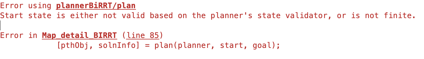
[pthObj, solnInfo] = plan(planner, start, goal);
smoothWaypointsObj = exampleHelperUAVPathSmoothing(ss, sv, pthObj);
distances(i, j) = pathLength(smoothWaypointsObj);
end
end
end
toc
and the error below
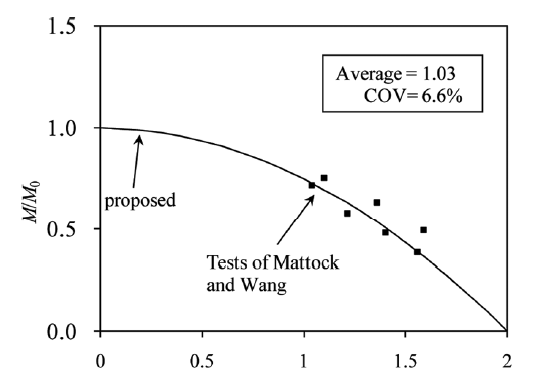 Hi, I have this equation for moment-axial force interaction: 0.25*(M/M0)^2 + (N/N0) = 1. This equation produces the following curve. Now, I need to make a change to this equation so that the first term becomes (M/M0)^2, and the second term can be changed while keeping (N/N0). The other side of the equation remains the same. ((M/M0)^2+?? = 1). I need to get the same curve as in the figure.
Hello everyone,
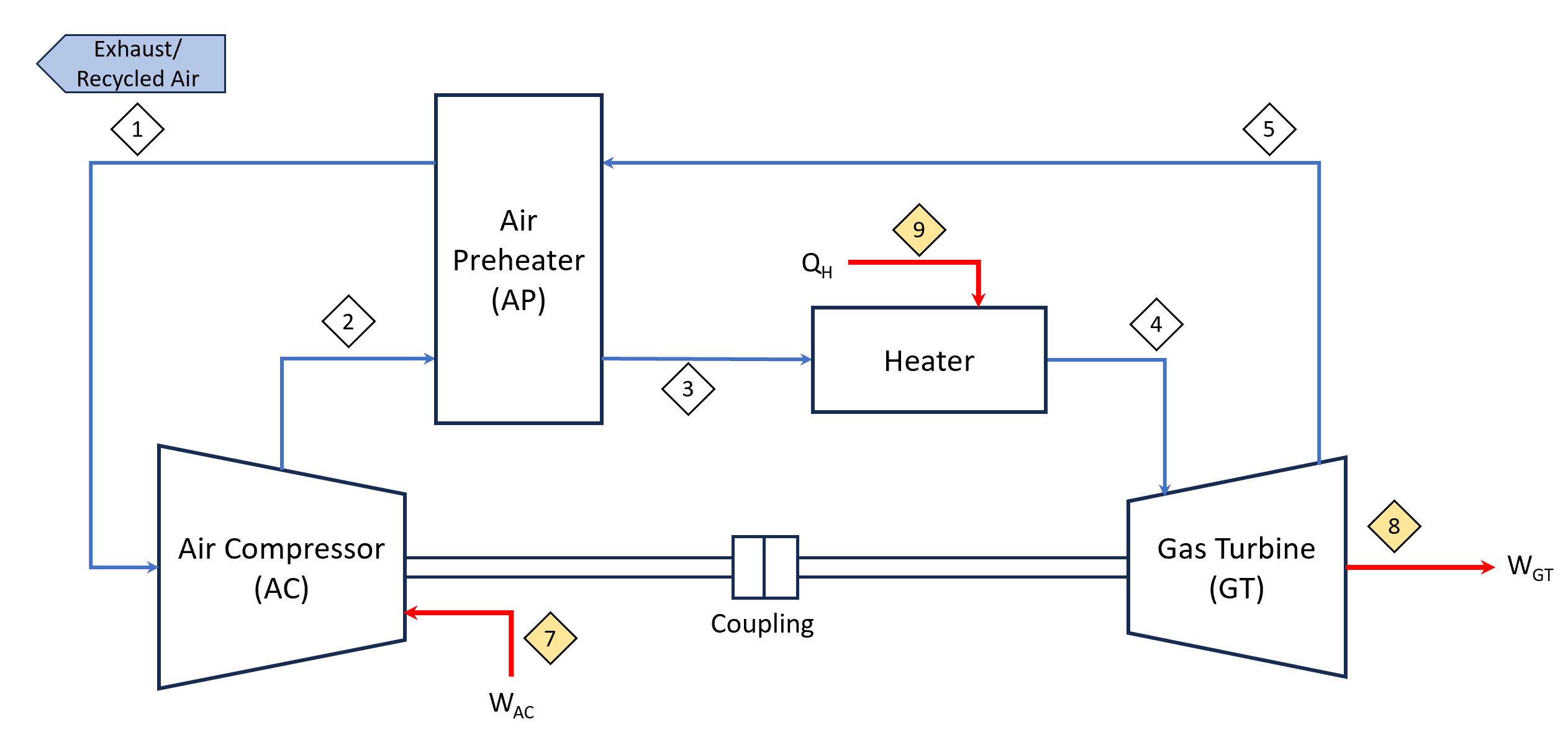
I am trying simulate a gas turbine system for my course on modelling and optimization of energy system. I have come out with a design consisting of a compressor, air preheater, combustion chamber and gas turbine. When I try to do the modelling in Simulink, I couldnt find something similar to combustion chamber. Does anyone have any experience in doing this?
Orginal Design:
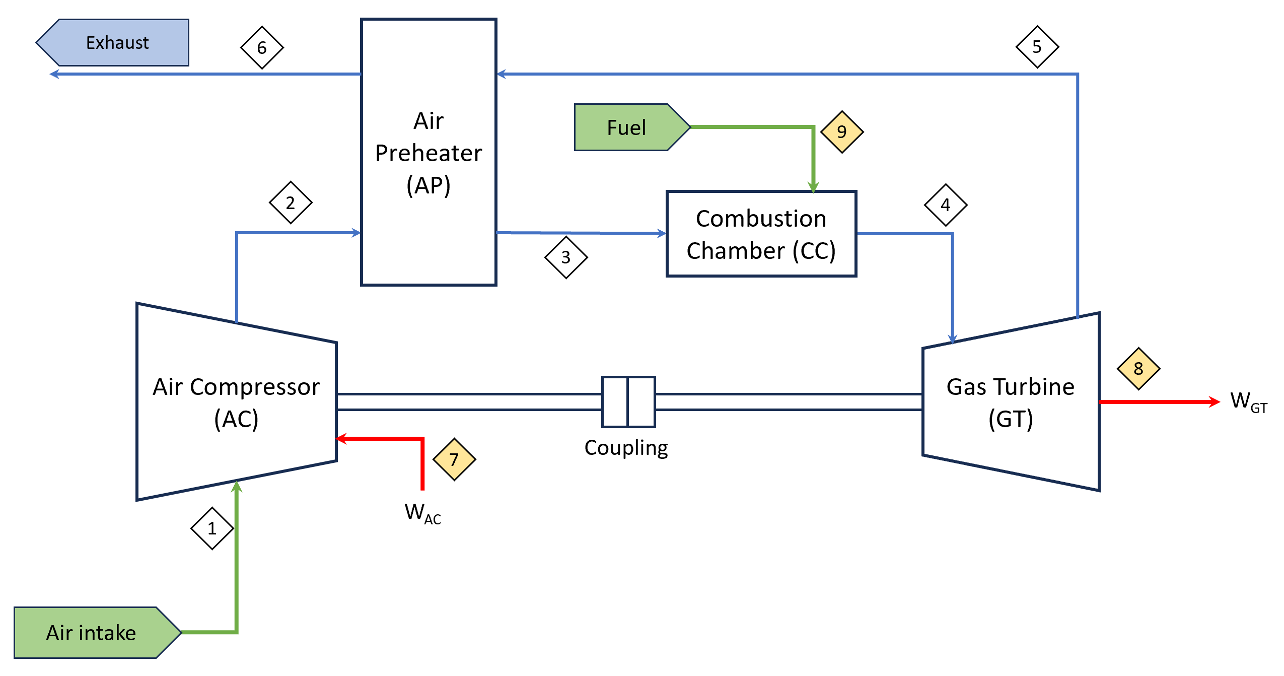
I have also amended it and come out with second design, where I change to combustion chamber to a heater and the exhaust air is recycled back to air compressor, making it a closed loop system. But I am also unable to find heater from the simulink library, the closest i can get is convective heat transfer. Can someone help on this too and if the closed loop system is feasible to model?
Design 2 :
Hi everyone,
for my thesis project I would need to get, every second of the simulation, real-time output data from a Simulink model, without using Simulink Real-Time, as it supports only Speedgoat Hardware. Is there a particular set of blocks for that purpose?
I have to provide that real-time data to hardware for an Hardware in the Loop Simulation so I will need to be able also to receive, as an input, data from the hardware to the Simulink model, again every second of the simulation, to close the loop of the simulation.
Thank you in advance for your support.
Hi! I am using matlab inbuilt plot option( without typing code) to plot the data. This joins the data points using straight line by default. What will be the easiest way to plot if I want curve to join the points instead?
I keep getting this error message when trying to run my code, I'm confident my wiring is correct and I do not know what this error means-
Library 'Servo' is not uploaded to the board. Clear the current Arduino object and recreate it to include the appropriate library. For a list of available libraries, type 'listArduinoLibraries'.
here is my code
a=arduino();
s1 = servo(a, 'D9', 'MinPulseDuration', 700*10^-6, 'MaxPulseDuration', 2300*10^-6);
writePosition(s1,0);
userResponse = "yes";
while userResponse == "yes"
chicken = input("Insert your resistor");
voltage = readVoltage(a, "A0");
if voltage < 1.67155
resistor = "47k";
writePosition(s1,0.25);
minR = 47000 * 0.95;
maxR = 47000 * 1.05;
elseif voltage < 3.53128
resistor = "10k";
writePosition(s1,0.5);
minR = 10000 * 0.95;
maxR = 10000 * 1.05;
elseif voltage < 4.69941
resistor = "1k";
writePosition(s1,0.75);
minR = 1000 * 0.95;
maxR = 1000 * 1.05;
else
resistor = "330";
writePosition(s1,1);
minR = 330 * 0.95;
maxR = 330 * 1.05;
end
resistance = voltageToResistance(voltage);
withinTolerance = (resistance >= minR && resistance <= maxR);
disp(resistor)
if withinTolerance == 1
writeDigitalPin(a, "D4", 1);
writeDigitalPin(a, "D5", 0);
%disp("green")
else
writeDigitalPin(a, "D4", 0);
writeDigitalPin(a, "D5", 1);
%disp("Red")
end
userResponse = input("Would you like to check another resistor? ","s");
writePosition(s1,0);
writeDigitalPin(a, "D4", 0);
writeDigitalPin(a, "D5", 0);
end
How to Simulate a Synchronous Compensator in Simulink?
We are thrilled to announce the grand prize winners of our MATLAB Flipbook contest! This year, we invited the MATLAB Graphics Infrastructure team, renowned for their expertise in exporting and animation workflows, to be our judges. After careful consideration, they have selected the top three winners:
Judge comments: Creative and realistic rendering with well-written code
2nd place - Christmas Tree / Zhaoxu Liu
Judge comments: Festive and advanced animation that is appropriate to the current holiday season.
Judge comments: Nice translation of existing shader logic to MATLAB that produces an advanced and appealing visual effect.
In addition, after validating the votes, we are pleased to announce the top 10 participants on the leaderboard:
- Tim
- Zhaoxu Liu / slandarer
- KARUPPASAMYPANDIYAN M
- Dhimas Mahardika S.Si., M.Mat
- Augusto Mazzei
- Jenny Bosten
- Lucas
- Jr
- Victoria
- ME
Congratulations to all! Your creativity and skills have inspired many of us to explore and learn new skills, and make this contest a big success!