Results for
Bringing the beauty of MathWorks Natick's tulips to life through code!
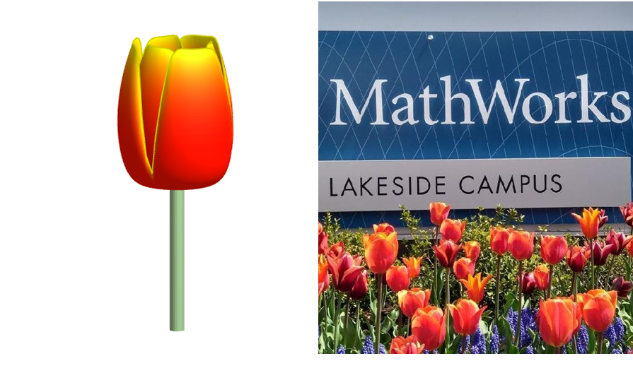
Remix challenge: create and share with us your new breeds of MATLAB tulips!
Hello MATLAB community,
I am doing some image processing with MATLAB and some issues with my coding. I just like to warn you that I am very new at coding and MATLAB so I apologise in advance for my low level and I would be very glad to have some help as I have hitted a wall, and can't find a solution to my problem.
Context: I have a video of beams, that move right to left over time. The base is fixed, only the beam moves. I converted the video to images, and my MATLAB program is going through the image file and treating every image in it. Here are two image examples:
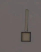 and
and 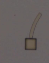
I want to measure the following things:
a. The coordinates between the 2 extremities of the beam (length of the beam, without its base), let's call them A and B.
b. The bending deformation E (L0-Lt/L0 *100), obtained by calculating the distance between A and B, called Lt.
c. the curvature of the beam (1/R), obtained by extracting the radius R of a circle fitting the curvature of the beam.
d. The angle between a vertical line passing through A, and the line AB.
What I have done so far:
My approach has been to transform my image into an rgbimage, then binaryImage, then have the complementary image, apply some modifications/corrections to the image, and then skeletonize it. And from then, I extract the coordinates of A and B, the distance between A&B (Lt), the radius of the beam R, and the angle between A&B (T).
My main issue is the skeletonisation. Because my beam is quite thick, it shortens up too much my beam, and in an inconcistent manner. So then my results are completly wrong. Here is an image of the different images and operation I have done and the result:
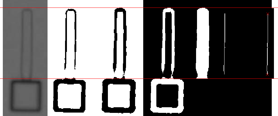
So as you can see, the length is shorter. I would like to have a skeleton that meets the edges of the beam to calculate the end points.
I have tried "bwskel(BW, 'MinBranchLength', 30)" and "bwmorph(BW, 'thin', inf)", and this: https://uk.mathworks.com/matlabcentral/fileexchange/11123-better-skeletonization. But the problem remains the same. I have tried regionpropos, but the major axis they return is too long, I have tried bwferet(), but the maxlength is in diagonal of the beam... I have running out of ideas.
Problem: So I guess my main problem is how can I get a skeletonisation that goes to the edges of the beam?
Here is my code:
for i = TrackingStart:TrackingEnd
FileRGB(:,:,i) = rgb2gray(imread(IMG)); % Convert to grayscale
croppedRGB = FileRGB(y3left:y3right, x3left:x3right, i);
binaryImage = imbinarize(croppedRGB, 'adaptive', 'ForegroundPolarity','dark','Sensitivity', 0.50);
out = nnz(~binaryImage);
while out <= 4300 % Change threshold if needed
for j = 1:50
sensitivity = 0.50 + j * 0.01;
binaryImage = imbinarize(croppedRGB, 'adaptive', 'ForegroundPolarity', 'dark', 'Sensitivity', sensitivity);
out = nnz(~binaryImage);
if out >= 4325
break; % Exit the loop if the condition is met
end
end
end
% Create a line Model
BW = imcomplement(binaryImage);
BW(y1left:y1right, x1left:x1right) = 1; % there is always sample at the junction area (between beam and base)
BW(y2left:y2right, x2left:x2right) = 0; % Always = 0 if no sample here
BW = bwmorph(BW, 'close', Inf);
BW = bwmorph(BW, 'bridge');
BW = bwareafilt(BW, 1);
s = regionprops(BW, 'FilledImage');
BW = s.FilledImage;
BW = bwskel(BW, 'MinBranchLength', 30);
endpoints = bwmorph(BW, 'endpoints');
[y_end, x_end] = find(endpoints == 1);
%Degree of bending deformation method
Lt = sqrt(power(x_end(1)-x_end(2),2)+power(y_end(1)-y_end(2),2));
if x_end(2) > x_end(1)
Lt = -Lt;
end
Lstore(i) = Lt;
%Curvature method
[row_dots_cir, col_dots_cir, val] = find(BW == 1);
[xc(i),yc(i),Rstore(i),a] = circfit(col_dots_cir,row_dots_cir);
%Angle method
slope_endpoints = (x_end(1) - x_end(2)) / (y_end(1) - y_end(2));
angle_radians = atan(slope_endpoints);
angle_degrees = rad2deg(angle_radians);
if x_end(2) > x_end(1)
angle_degrees = -angle_degrees;
end
Tstore(i) = angle_degrees;
i
end
I found this plot of words said by different characters on the US version of The Office sitcom. There's a sparkline for each character from pilot to finale episode.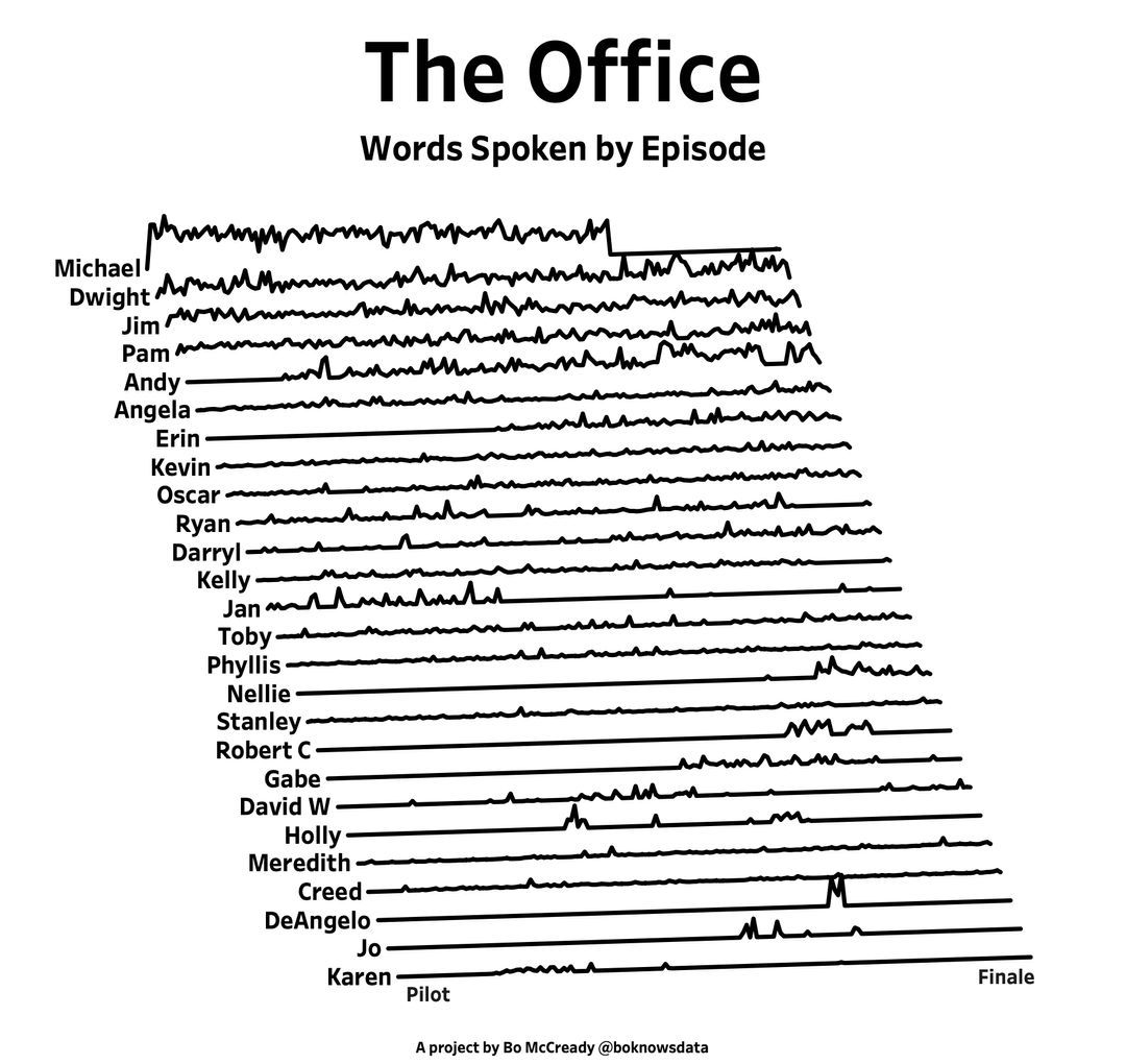
RGB triplet [0,1]
9%
RGB triplet [0,255]
12%
Hexadecimal Color Code
13%
Indexed color
16%
Truecolor array
37%
Equally unfamiliar with all-above
13%
2784 votes
A high school student called for help with this physics problem:
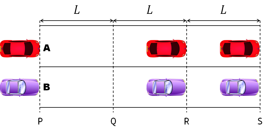
- Car A moves with constant velocity v.
- Car B starts to move when Car A passes through the point P.
- Car B undergoes...
- uniform acc. motion from P to Q.
- uniform velocity motion from Q to R.
- uniform acc. motion from R to S.
- Car A and B pass through the point R simultaneously.
- Car A and B arrive at the point S simultaneously.
Q1. When car A passes the point Q, which is moving faster?
Q2. Solve the time duration for car B to move from P to Q using L and v.
Q3. Magnitude of acc. of car B from P to Q, and from R to S: which is bigger?
Well, it can be solved with a series of tedious equations. But... how about this?
Code below:
%% get images and prepare stuffs
figure(WindowStyle="docked"),
ax1 = subplot(2,1,1);
hold on, box on
ax1.XTick = [];
ax1.YTick = [];
A = plot(0, 1, 'ro', MarkerSize=10, MarkerFaceColor='r');
B = plot(0, 0, 'bo', MarkerSize=10, MarkerFaceColor='b');
[carA, ~, alphaA] = imread('https://cdn.pixabay.com/photo/2013/07/12/11/58/car-145008_960_720.png');
[carB, ~, alphaB] = imread('https://cdn.pixabay.com/photo/2014/04/03/10/54/car-311712_960_720.png');
carA = imrotate(imresize(carA, 0.1), -90);
carB = imrotate(imresize(carB, 0.1), 180);
alphaA = imrotate(imresize(alphaA, 0.1), -90);
alphaB = imrotate(imresize(alphaB, 0.1), 180);
carA = imagesc(carA, AlphaData=alphaA, XData=[-0.1, 0.1], YData=[0.9, 1.1]);
carB = imagesc(carB, AlphaData=alphaB, XData=[-0.1, 0.1], YData=[-0.1, 0.1]);
txtA = text(0, 0.85, 'A', FontSize=12);
txtB = text(0, 0.17, 'B', FontSize=12);
yline(1, 'r--')
yline(0, 'b--')
xline(1, 'k--')
xline(2, 'k--')
text(1, -0.2, 'Q', FontSize=20, HorizontalAlignment='center')
text(2, -0.2, 'R', FontSize=20, HorizontalAlignment='center')
% legend('A', 'B') % this make the animation slow. why?
xlim([0, 3])
ylim([-.3, 1.3])
%% axes2: plots velocity graph
ax2 = subplot(2,1,2);
box on, hold on
xlabel('t'), ylabel('v')
vA = plot(0, 1, 'r.-');
vB = plot(0, 0, 'b.-');
xline(1, 'k--')
xline(2, 'k--')
xlim([0, 3])
ylim([-.3, 1.8])
p1 = patch([0, 0, 0, 0], [0, 1, 1, 0], [248, 209, 188]/255, ...
EdgeColor = 'none', ...
FaceAlpha = 0.3);
%% solution
v = 1; % car A moves with constant speed.
L = 1; % distances of P-Q, Q-R, R-S
% acc. of car B for three intervals
a(1) = 9*v^2/8/L;
a(2) = 0;
a(3) = -1;
t_BatQ = sqrt(2*L/a(1)); % time when car B arrives at Q
v_B2 = a(1) * t_BatQ; % speed of car B between Q-R
%% patches for velocity graph
p2 = patch([t_BatQ, t_BatQ, t_BatQ, t_BatQ], [1, 1, v_B2, v_B2], ...
[248, 209, 188]/255, ...
EdgeColor = 'none', ...
FaceAlpha = 0.3);
p3 = patch([2, 2, 2, 2], [1, v_B2, v_B2, 1], [194, 234, 179]/255, ...
EdgeColor = 'none', ...
FaceAlpha = 0.3);
%% animation
tt = linspace(0, 3, 2000);
for t = tt
A.XData = v * t;
vA.XData = [vA.XData, t];
vA.YData = [vA.YData, 1];
if t < t_BatQ
B.XData = 1/2 * a(1) * t^2;
vB.XData = [vB.XData, t];
vB.YData = [vB.YData, a(1) * t];
p1.XData = [0, t, t, 0];
p1.YData = [0, vB.YData(end), 1, 1];
elseif t >= t_BatQ && t < 2
B.XData = L + (t - t_BatQ) * v_B2;
vB.XData = [vB.XData, t];
vB.YData = [vB.YData, v_B2];
p2.XData = [t_BatQ, t, t, t_BatQ];
p2.YData = [1, 1, vB.YData(end), vB.YData(end)];
else
B.XData = 2*L + v_B2 * (t - 2) + 1/2 * a(3) * (t-2)^2;
vB.XData = [vB.XData, t];
vB.YData = [vB.YData, v_B2 + a(3) * (t - 2)];
p3.XData = [2, t, t, 2];
p3.YData = [1, 1, vB.YData(end), v_B2];
end
txtA.Position(1) = A.XData(end);
txtB.Position(1) = B.XData(end);
carA.XData = A.XData(end) + [-.1, .1];
carB.XData = B.XData(end) + [-.1, .1];
drawnow
end
I have question about using 'bnlssm' object when the problem involves time-varying coefs. Per this documentation https://www.mathworks.com/help/econ/bnlssm.html , bnlssm allows the transition matrix to be a nonlinear function of the past values of the state vector, while also being time-varying --, i.e. A_t(x_{t-1}). However the documentation contains an example of the parameter mapping function for a fixed coef. case only:
function [A,B,C,D,Mean0,Cov0,StateType] = paramMap(theta)
A = @(x)blkdiag([theta(1) theta(2); 0 1],[theta(3) theta(4); 0 1])*x;
B = [theta(5) 0; 0 0; 0 theta(6); 0 0];
C = @(x)log(exp(x(1)-theta(2)/(1-theta(1))) + ...
exp(x(3)-theta(4)/(1-theta(3))));
D = theta(7);
Mean0 = [theta(2)/(1-theta(1)); 1; theta(4)/(1-theta(3)); 1];
Cov0 = diag([theta(5)^2/(1-theta(1)^2) 0 theta(6)^2/(1-theta(3)^2) 0]);
StateType = [0; 1; 0; 1]; % Stationary state and constant 1 processes
end
Here, A and C are recognised as function handles and show the dimension of 1-by-1 when [A,B,C,D]=paramMap(theta) is run with a given theta. This does not prevent filter/smooth from returning the states estimates, as the function handles become m-by-m matices when the function handles are evaluated.
However, whenever I try replaceing A with a cell array, e.g.:
A=cell(T,1);
for t=1:T
A{t} = @(x)blkdiag([theta(1) theta(2); 0 1],[theta(3) theta(4); 0 1])*x;
end
bnlssm.fixcoeff throws an error that the dimensions of Mean0 are expected to be 1, per validation step in lines 700-707 of 'bnlssm.m':
if iscellA; At = A{1};
else; At = A; end
numStates0 = size(At,2);
if
isscalar(mean0)
mean0 = mean0(ones(numStates0,1),:);
elseif
~isempty(mean0)
mean0 = mean0(:);
validateattributes(mean0,{'numeric'},{'finite','real','numel',numStates0},callerName,'Mean0');
end
Q: Is it just overlook by MathWorks programmers and creating local verions of bnlssm/filter/smooth with that validation step removed is a viable pathway forward, or is it intentional because 'bnlssm' was in fact designed to handle only the time-invariant coef. case correctly?
%%https://in.mathworks.com/matlabcentral/cody/problems/3-find-the-sum-of-all-the-numbers-of-the-input-vector/solutions/new#
%Above is the complete link of question that is ask and below i am providing my code for %this problem, please guide how do i rearrange this so that i can pass all the test at a time.
function y = vecsum(x)
x= 1:100;
y1= sum(x(1,[1]));
y2= sum(x(1,[1 2 3 5]));
y3= sum(x);
y=[y1 y2 y3];
end
Are you a Simulink user eager to learn how to create apps with App Designer? Or an App Designer enthusiast looking to dive into Simulink?
Don't miss today's article on the Graphics and App Building Blog by @Robert Philbrick! Discover how to build Simulink Apps with App Designer, streamlining control of your simulations!
Hi All,
I'm trying to get code coverage analysis report while cosimulation of generated HDL code through Questasim in Simulink. I'm getting blank results in coverage analysis section of Questasim. Can you please help me to get code coverage details ? Thanks in Advance.
Matlab: 2022b
Questasim: 2020.1
Northern lights captured from this weekend at MathWorks campus ✨
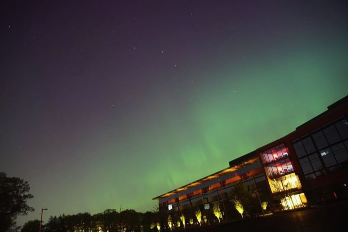
Did you get a chance to see lights and take some photos?
From Alpha Vantage's website: API Documentation | Alpha Vantage
Try using the built-in Matlab function webread(URL)... for example:
% copy a URL from the examples on the site
URL = 'https://www.alphavantage.co/query?function=TIME_SERIES_DAILY&symbol=IBM&apikey=demo'
% or use the pattern to create one
tickers = [{'IBM'} {'SPY'} {'DJI'} {'QQQ'}]; i = 1;
URL = ...
['https://www.alphavantage.co/query?function=TIME_SERIES_DAILY_ADJUSTED&outputsize=full&symbol=', ...
+ tickers{i}, ...
+ '&apikey=***Put Your API Key here***'];
X = webread(URL);
You can access any of the data available on the site as per the Alpha Vantage documentation using these two lines of code but with different designations for the requested data as per the documentation.
It's fun!
isstring
11%
ischar
7%
iscellstr
13%
isletter
21%
isspace
9%
ispunctuation
37%
2455 votes
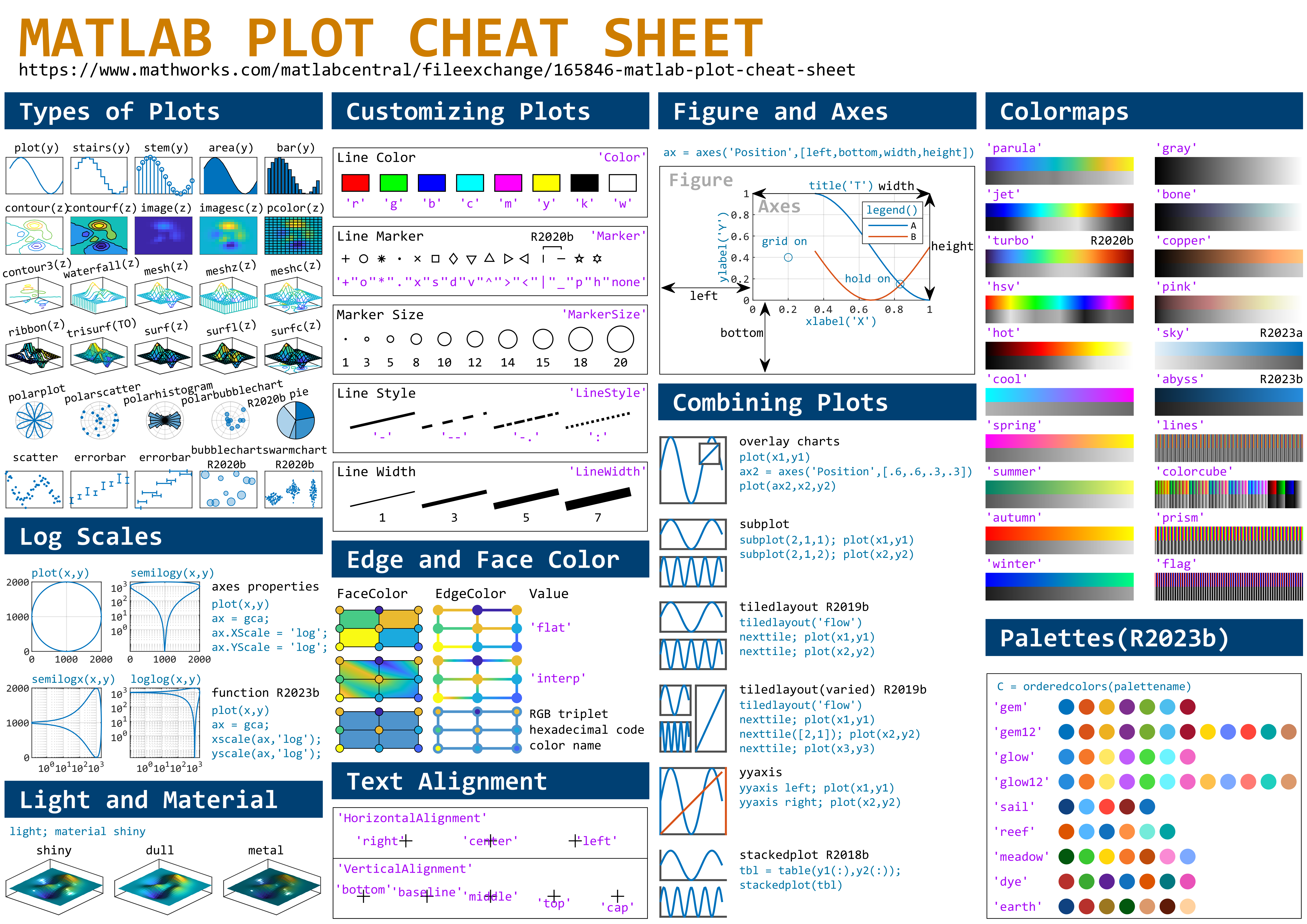
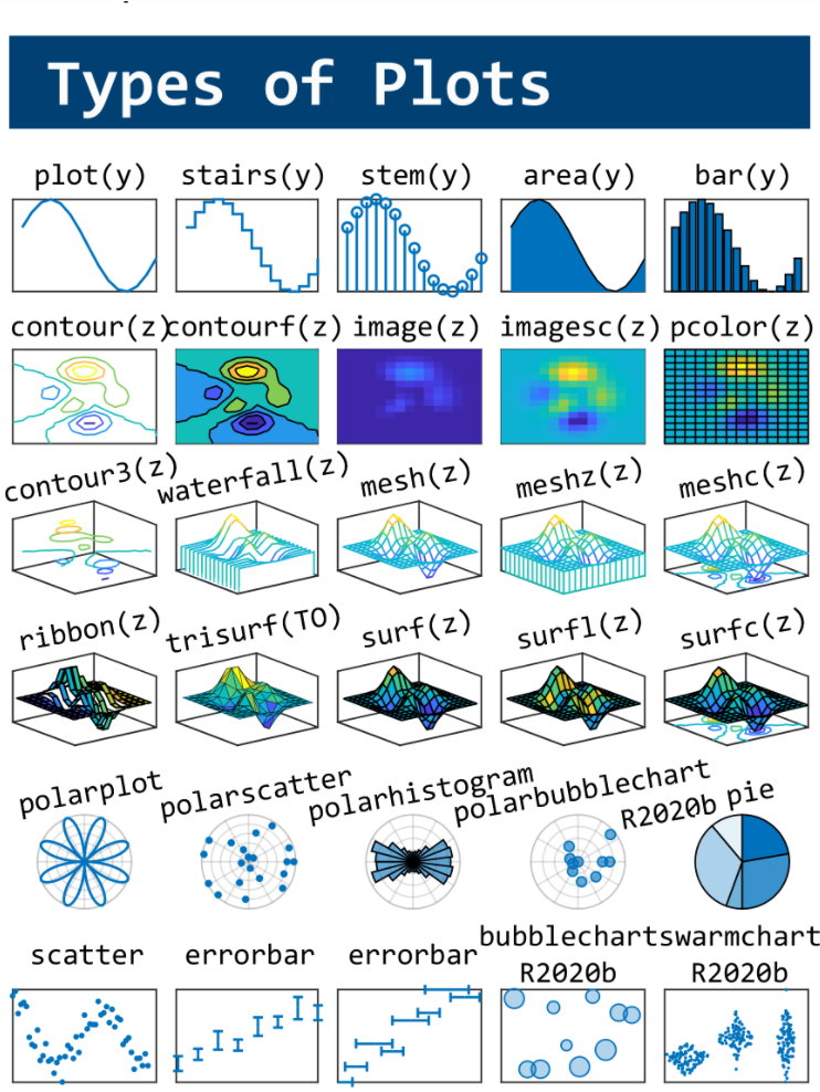
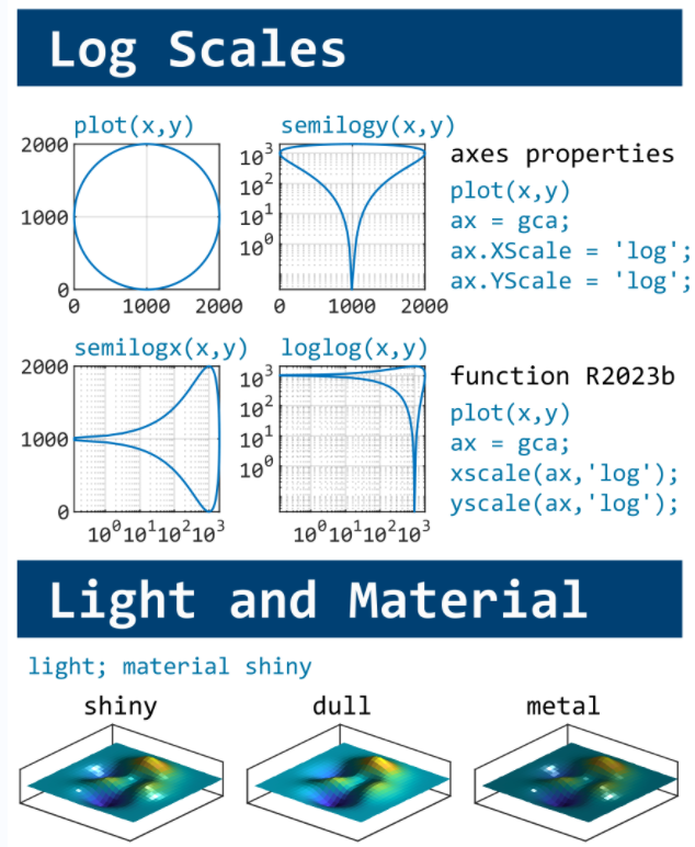
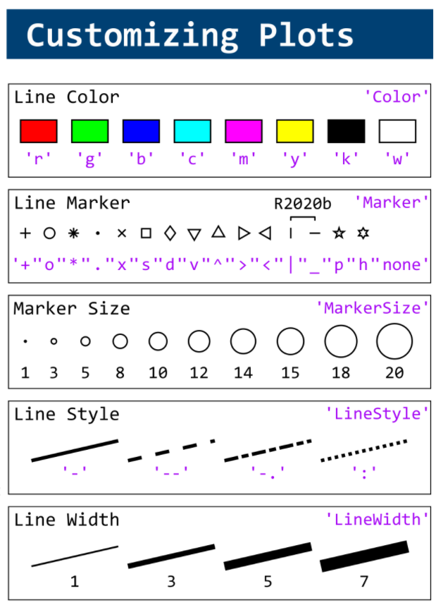
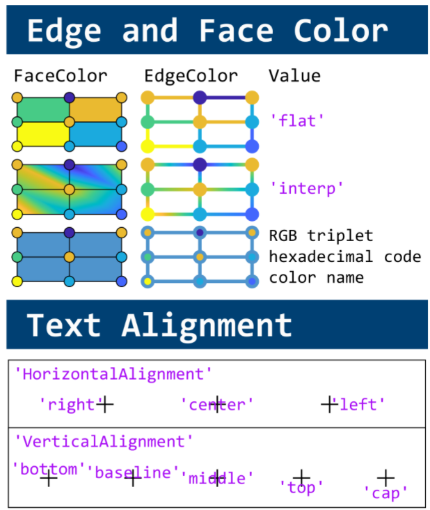
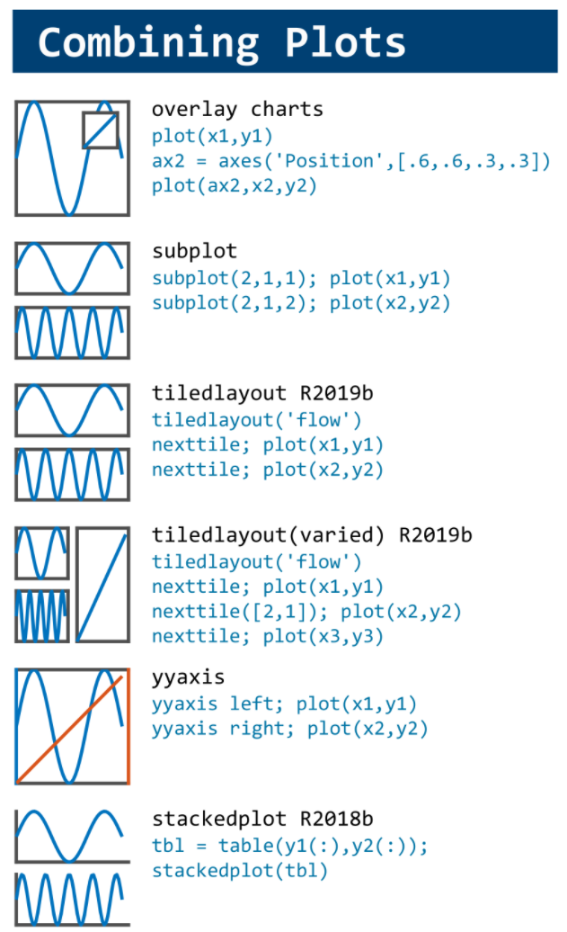
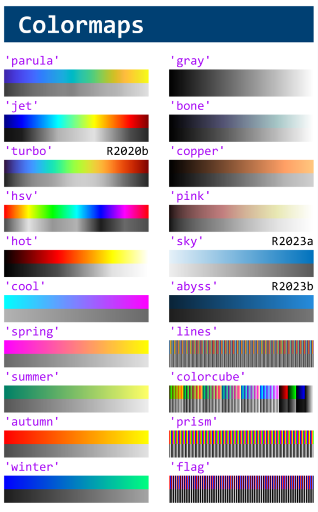
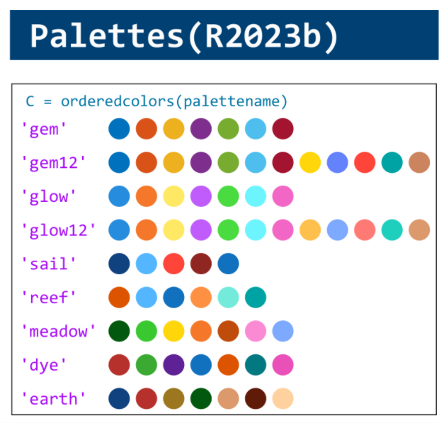
This cheat sheet is here:
reference:
- https://github.com/peijin94/matlabPlotCheatsheet
- https://github.com/mathworks/visualization-cheat-sheet
- https://www.mathworks.com/products/matlab/plot-gallery.html
- https://www.mathworks.com/help/matlab/release-notes.html
MATLAB used to have official visualization-cheat-sheet, but there have been quite a few new updates in MATLAB versions recently. Therefore, I made my own cheat sheet and marked the versions of each new thing that were released :
Hi to all.
I'm trying to learn a bit about trading with cryptovalues. At the moment I'm using Freqtrade (in dry-run mode of course) for automatic trading. The tool is written in python and it allows to create custom strategies in python classes and then run them.
I've written some strategy just to learn how to do, but now I'd like to create some interesting algorithm. I've a matlab license, and I'd like to know what are suggested tollboxes for following work:
- Create a criptocurrency strategy algorythm (for buying and selling some crypto like BTC, ETH etc).
- Backtesting the strategy with historical data (I've a bunch of json files with different timeframes, downloaded with freqtrade from binance).
- Optimize the strategy given some parameters (they can be numeric, like ROI, some kind of enumeration, like "selltype" and so on).
- Convert the strategy algorithm in python, so I can use it with Freqtrade without worrying of manually copying formulas and parameters that's error prone.
- I'd like to write both classic algorithm and some deep neural one, that try to find best strategy with little neural network (they should run on my pc with 32gb of ram and a 3080RTX if it can be gpu accelerated).
What do you suggest?
If structure is in the form of struct1.struct2(m,n).struct3. how to extract values present in struct3 using mex function
Dear MATLAB contest enthusiasts,
I believe many of you have been captivated by the innovative entries from Zhaoxu Liu / slanderer, in the 2023 MATLAB Flipbook Mini Hack contest.

Ever wondered about the person behind these creative entries? What drives a MATLAB user to such levels of skill? And what inspired his participation in the contest? We were just as curious as you are!
We were delighted to catch up with him and learn more about his use of MATLAB. The interview has recently been published in MathWorks Blogs. For an in-depth look into his insights and experiences, be sure to read our latest blog post: Community Q&A – Zhaoxu Liu.
But the conversation doesn't end here! Who would you like to see featured in our next interview? Drop their name in the comments section below and let us know who we should reach out to next!
Hey MATLAB Community! 🌟
In the vibrant landscape of our online community, the past few weeks have been particularly exciting. We've seen a plethora of contributions that not only enrich our collective knowledge but also foster a spirit of collaboration and innovation. Here are some of the noteworthy contributions from our members.
Interesting Questions
Victor encountered a puzzling error while trying to publish his script to PDF. His post sparked a helpful discussion on troubleshooting this issue, proving invaluable for anyone facing similar challenges.
Devendra's inquiry into interpolating and smoothing NDVI time series using MATLAB has opened up a dialogue on various techniques to manage noisy data, benefiting researchers and enthusiasts in the field of remote sensing.
Popular Discussions
Adam Danz's AMA session has been a treasure trove of insights into the workings behind the MATLAB Answers forum, offering a unique perspective from a staff contributor's viewpoint.
The User Following feature marks a significant enhancement in how community members can stay connected with the contributions of their peers, fostering a more interconnected MATLAB Central.
From File Exchange
Robert Haaring's submission is a standout contribution, providing a sophisticated model for CO2 electrolysis, a topic of great relevance to researchers in environmental technology and chemical engineering.
From the Blogs
Verification and Validation for AI: From model implementation to requirements validation by Sivylla Paraskevopoulou
Sivylla's comprehensive post delves into the critical stages of AI model development, from implementation to validation, offering invaluable guidance for professionals navigating the complexities of AI verification.
In this engaging Q&A, Ned Gulley introduces us to Zhaoxu Liu, a remarkable community member whose innovative contributions and active engagement have left a significant impact on the MATLAB community.
Each of these contributions highlights the diverse and rich expertise within our community. From solving complex technical issues to introducing new features and sharing in-depth knowledge on specialized topics, our members continue to make MATLAB Central a vibrant and invaluable resource.
Let's continue to support, inspire, and learn from one another
Don't use / What are Projects?
26%
1–10
31%
11–20
15%
21–30
9%
31–50
7%
51+ (comment below)
12%
4070 votes
The study of the dynamics of the discrete Klein - Gordon equation (DKG) with friction is given by the equation :

above equation, W describes the potential function :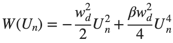
The objective of this simulation is to model the dynamics of a segment of DNA under thermal fluctuations with fixed boundaries using a modified discrete Klein-Gordon equation. The model incorporates elasticity, nonlinearity, and damping to provide insights into the mechanical behavior of DNA under various conditions.
% Parameters
numBases = 200; % Number of base pairs, representing a segment of DNA
kappa = 0.1; % Elasticity constant
omegaD = 0.2; % Frequency term
beta = 0.05; % Nonlinearity coefficient
delta = 0.01; % Damping coefficient
- Position: Random initial perturbations between 0.01 and 0.02 to simulate the thermal fluctuations at the start.
- Velocity: All bases start from rest, assuming no initial movement except for the thermal perturbations.
% Random initial perturbations to simulate thermal fluctuations
initialPositions = 0.01 + (0.02-0.01).*rand(numBases,1);
initialVelocities = zeros(numBases,1); % Assuming initial rest state
The simulation uses fixed ends to model the DNA segment being anchored at both ends, which is typical in experimental setups for studying DNA mechanics. The equations of motion for each base are derived from a modified discrete Klein-Gordon equation with the inclusion of damping:
% Define the differential equations
dt = 0.05; % Time step
tmax = 50; % Maximum time
tspan = 0:dt:tmax; % Time vector
x = zeros(numBases, length(tspan)); % Displacement matrix
x(:,1) = initialPositions; % Initial positions
% Velocity-Verlet algorithm for numerical integration
for i = 2:length(tspan)
% Compute acceleration for internal bases
acceleration = zeros(numBases,1);
for n = 2:numBases-1
acceleration(n) = kappa * (x(n+1, i-1) - 2 * x(n, i-1) + x(n-1, i-1)) ...
- delta * initialVelocities(n) - omegaD^2 * (x(n, i-1) - beta * x(n, i-1)^3);
end
% positions for internal bases
x(2:numBases-1, i) = x(2:numBases-1, i-1) + dt * initialVelocities(2:numBases-1) ...
+ 0.5 * dt^2 * acceleration(2:numBases-1);
% velocities using new accelerations
newAcceleration = zeros(numBases,1);
for n = 2:numBases-1
newAcceleration(n) = kappa * (x(n+1, i) - 2 * x(n, i) + x(n-1, i)) ...
- delta * initialVelocities(n) - omegaD^2 * (x(n, i) - beta * x(n, i)^3);
end
initialVelocities(2:numBases-1) = initialVelocities(2:numBases-1) + 0.5 * dt * (acceleration(2:numBases-1) + newAcceleration(2:numBases-1));
end
% Visualization of displacement over time for each base pair
figure;
hold on;
for n = 2:numBases-1
plot(tspan, x(n, :));
end
xlabel('Time');
ylabel('Displacement');
legend(arrayfun(@(n) ['Base ' num2str(n)], 2:numBases-1, 'UniformOutput', false));
title('Displacement of DNA Bases Over Time');
hold off;
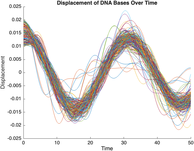
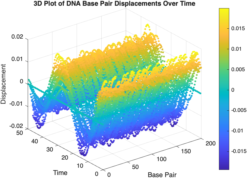
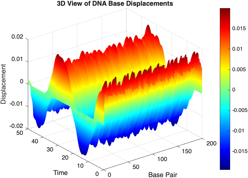
The results are visualized using a plot that shows the displacements of each base over time . Key observations from the simulation include :
- Wave Propagation: The initial perturbations lead to wave-like dynamics along the segment, with visible propagation and reflection at the boundaries.
- Damping Effects: The inclusion of damping leads to a gradual reduction in the amplitude of the oscillations, indicating energy dissipation over time.
- Nonlinear Behavior: The nonlinear term influences the response, potentially stabilizing the system against large displacements or leading to complex dynamic patterns.
% 3D plot for displacement
figure;
[X, T] = meshgrid(1:numBases, tspan);
surf(X', T', x);
xlabel('Base Pair');
ylabel('Time');
zlabel('Displacement');
title('3D View of DNA Base Displacements');
colormap('jet');
shading interp;
colorbar; % Adds a color bar to indicate displacement magnitude
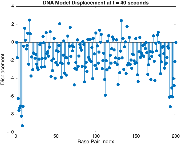
% Snapshot visualization at a specific time
snapshotTime = 40; % Desired time for the snapshot
[~, snapshotIndex] = min(abs(tspan - snapshotTime)); % Find closest index
snapshotSolution = x(:, snapshotIndex); % Extract displacement at the snapshot time
% Plotting the snapshot
figure;
stem(1:numBases, snapshotSolution, 'filled'); % Discrete plot using stem
title(sprintf('DNA Model Displacement at t = %d seconds', snapshotTime));
xlabel('Base Pair Index');
ylabel('Displacement');
% Time vector for detailed sampling
tDetailed = 0:0.5:50; % Detailed time steps
% Initialize an empty array to hold the data
data = [];
% Generate the data for 3D plotting
for i = 1:numBases
% Interpolate to get detailed solution data for each base pair
detailedSolution = interp1(tspan, x(i, :), tDetailed);
% Concatenate the current base pair's data to the main data array
data = [data; repmat(i, length(tDetailed), 1), tDetailed', detailedSolution'];
end
% 3D Plot
figure;
scatter3(data(:,1), data(:,2), data(:,3), 10, data(:,3), 'filled');
xlabel('Base Pair');
ylabel('Time');
zlabel('Displacement');
title('3D Plot of DNA Base Pair Displacements Over Time');
colorbar; % Adds a color bar to indicate displacement magnitude