Results for
How do you teach subjects like Programming and Numerical Computing hands-on in these challenging times?
Prof Chiranjoy Chattopadhyay at the Dept of Computer Science and Engineering at IIT Jodhpur shares his innovative approach to teaching at a distance in this new Technical Article on Teaching Parallel Computing Online with MATLAB.
The course utilized MATLAB Online , MATLAB Onramp and MATLAB Grader to train students in the basics of technical computing, in addition to using a Hands-on Online GPU workshop organised with the MathWorks Education Team. As a result of this approach to distance teaching, the students have reported good levels of understanding in the main learning outcomes of this course, as indicated in the survey results (below):

Please consider trying out the links above to check if your course might benefit from a similar approach, and feel free to message us if you are interested in learning more.
I just highlighted an app on File Exchange for emulating an experiment. Great idea for doing lab classes with software. What I like about this app is that it incorporates statistical variance and measurement noise that comes from physical experiments.
Read more about it here:
https://blogs.mathworks.com/pick/2020/11/20/emulating-a-physical-experiment-of-measuring-mms/
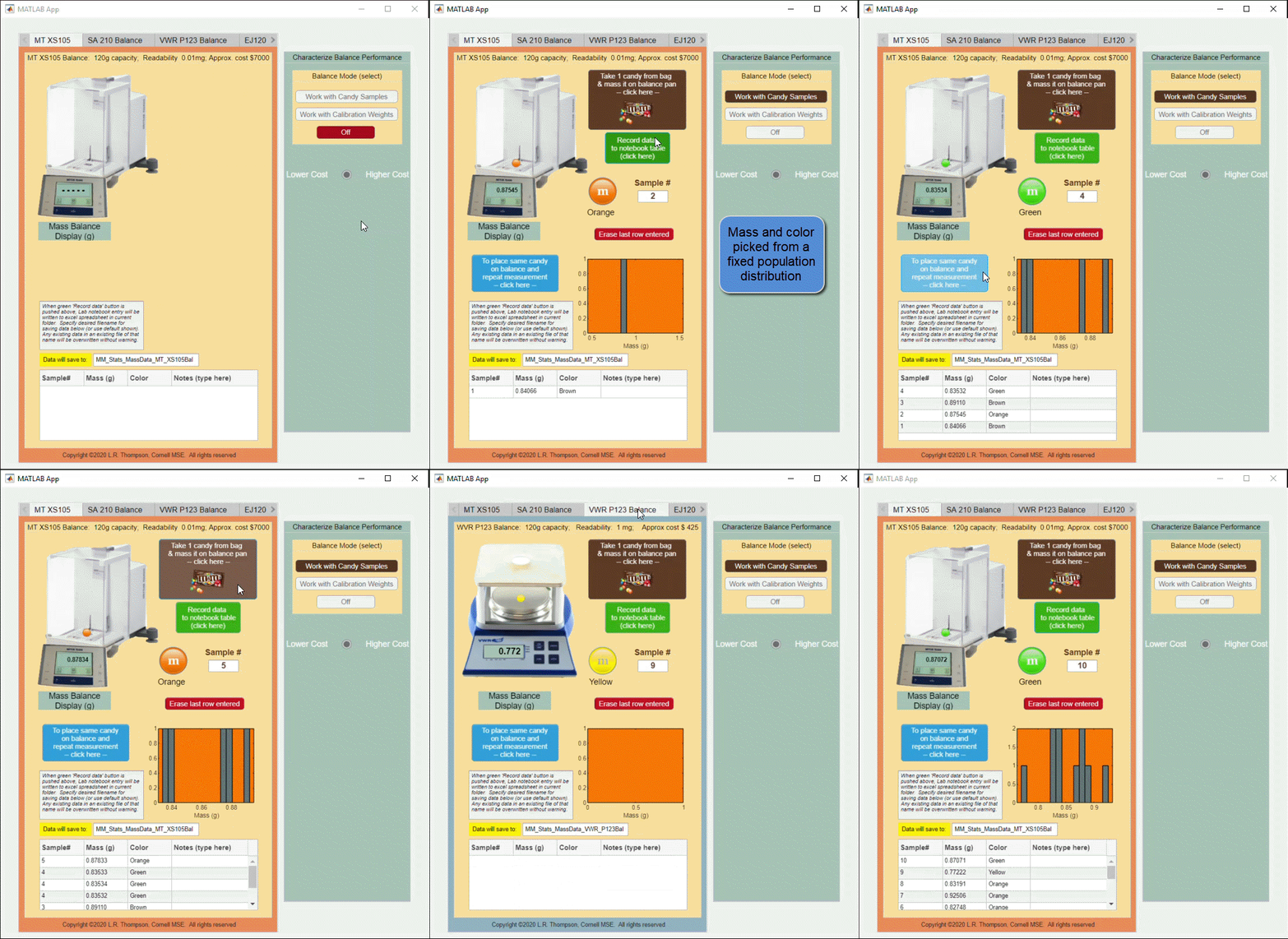
Emulating a physical experiment of measuring M&M’s
Jiro's Pick this week is M&M statistics by Lisa R. Thompson.A common challenge I hear from educators is how to conduct courses that involve experiments or some sort of hardware interactions during this pandemic. If students are not able to be present in the classroom where the instruments are then you may need to become creative in how you teach.
Hi everyone, I'm trying to estimate the Frequency Response of a buck converter. I've found this article: https://it.mathworks.com/company/newsletters/articles/estimating-the-frequency-response-of-a-power-electronics-model.html I've adapted the procedure to a buck converter and followed the instructions but something went wrong. In the last step I've performed a time-domain verification in a Simulink® simulation with the switch-mode buck converter and a Transfer Function block implementing the parametric estimation and compare the response of both systems to the same small perturbation signal but the estimated model response doesn't match the switching model response. I don't know why I've got a diverging systems. I've tried to reduce the load and modify the duty cycle but nothing changed. How can I fix it?
In the link below (File Exchange), you'll find an example with an electric motor supplied by a fuel cell stack (Simscape implementation) and a battery. When motor load is low-to-normal, the fuel cell provides excess energy, that is used to recharge the battery. At motor peak load, the battery needs to contribute in order to complete the expected duty. If you have any query or thoughts, please reach me at jsagardu@mathworks.com
https://www.mathworks.com/matlabcentral/fileexchange/59343-fuel-cell-battery-driven-electric-motor-h2-transfer
I would like to plot 2 discrete vectors on one graph created as follows: u=1; X={u,2*u,3*u,4*u,5*u,6*u,7*u,8*u,9*u}; Y={u,3*u,5*u,-u,-6*u,u-u,u^2,u^3,u^4}; stem(X,Y) unfortunately system returns error how to do it properly?
- Use the new exportapp function to capture an image of your app|uifigure
- MATLAB's getframe now supports apps & uifigures
- Review: How to get the handle to an app figure
Use the new exportapp function to capture an image of your app|uifigure
Imagine these scenarios:
- Your app contains several adjustable parameters that update an embedded plot and you'd like to remember the values of each app component so that you can recreate the plot with the same dataset
- You're constructing a manual for your app and would like to include images of your app
- You're app contains a process that automatically updates regularly and you'd like to store periodic snapshots of your app.
As of MATLABs R2020b release , we no longer must rely on 3rd party software to record an image of an app or uifigure.
exportapp(fig,filename) saves an image (JPEG | PNG | TIFF | PDF) of a uifigure ( fig) with the specified file name or full file path ( filename). MATLAB's documentation includes an example of how to add an [Export] button to an app that allows the user to select a path, filename, and extension for their exported image.
Here's another example that merely saves the image as a PDF to the app's main folder.
1. Add a button to the app and assign a ButtonPushed callback function to the button. This one also assigns an icon to the button in the form of an svg file.

2. Define the callback function to name the image after the app's name and include a datetime stamp. The image will be saved to the app's main folder.
% Button pushed function: SnapshotButton
function SnapshotButtonPushed(app, ~)
    % create filename containing the app's figure name (spaces removed)
    % and a datetime stamp in format yymmdd_hhmmss
    filename = sprintf('%s_%s.pdf',regexprep(app.MyApp.Name,' +',''), datestr(now(),'yymmdd_HHMMSS'));
    % Get the app's path
    filepath = fileparts(which([mfilename,'.mlapp']));
    % Store snapshot
    exportapp(app.MyApp, fullfile(filepath,filename))
end
Matlab's getframe now supports apps & uifigures
getframe(h) captures images of axes or a uifigure as a structure containing the image data which defines a movie frame. This function has been around for a while but as of r2020b , it now supports uifigures. By capturing consecutive frames, you can create a movie that can be played back within a Matlab figure (using movie ) or as an AVI file (using VideoWriter ). This is useful when demonstrating the effects of changes to app components.
The general steps to recording a process within an app as a movie are,
1. Add a button or some other event to your app that can invoke the frame recording process.
2. Animation is typically controlled by a loop with n iterations. Preallocate the structure array that will store the outputs to getframe. The example below stores the outputs within the app so that they are available by other functions within the app. That will require you to define the variable as a property in the app.
% nFrames is the number of iterations that will be recorded.
% recordedFrames is defined as a private property within the app
app.recordedFrames(1:nFrames) = struct('cdata',[],'colormap',[]);
3. Call getframe from within the loop that controls the animation. If you're using VideoWriter to create an AVI file, you'll also do that here (not shown, but see an example in the documentation ).
% app.myAppUIFigure: the app's figure handle
% getframe() also accepts axis handles
for i = 1:nFrames
... % code that updates the app for the next frame
      app.recordedFrames(i) = getframe(app.myAppUIFigure);
  end
4. Now the frame data are stored in app.recordedFrames and can be accessed from anywhere within the app. To play them back as a movie,
movie(app.recordedFrames)
% or
movie(app.recordedFrames, n) % to play the movie n-times
movie(app.recordedFrames, n, fps) % to specify the number of frames per second
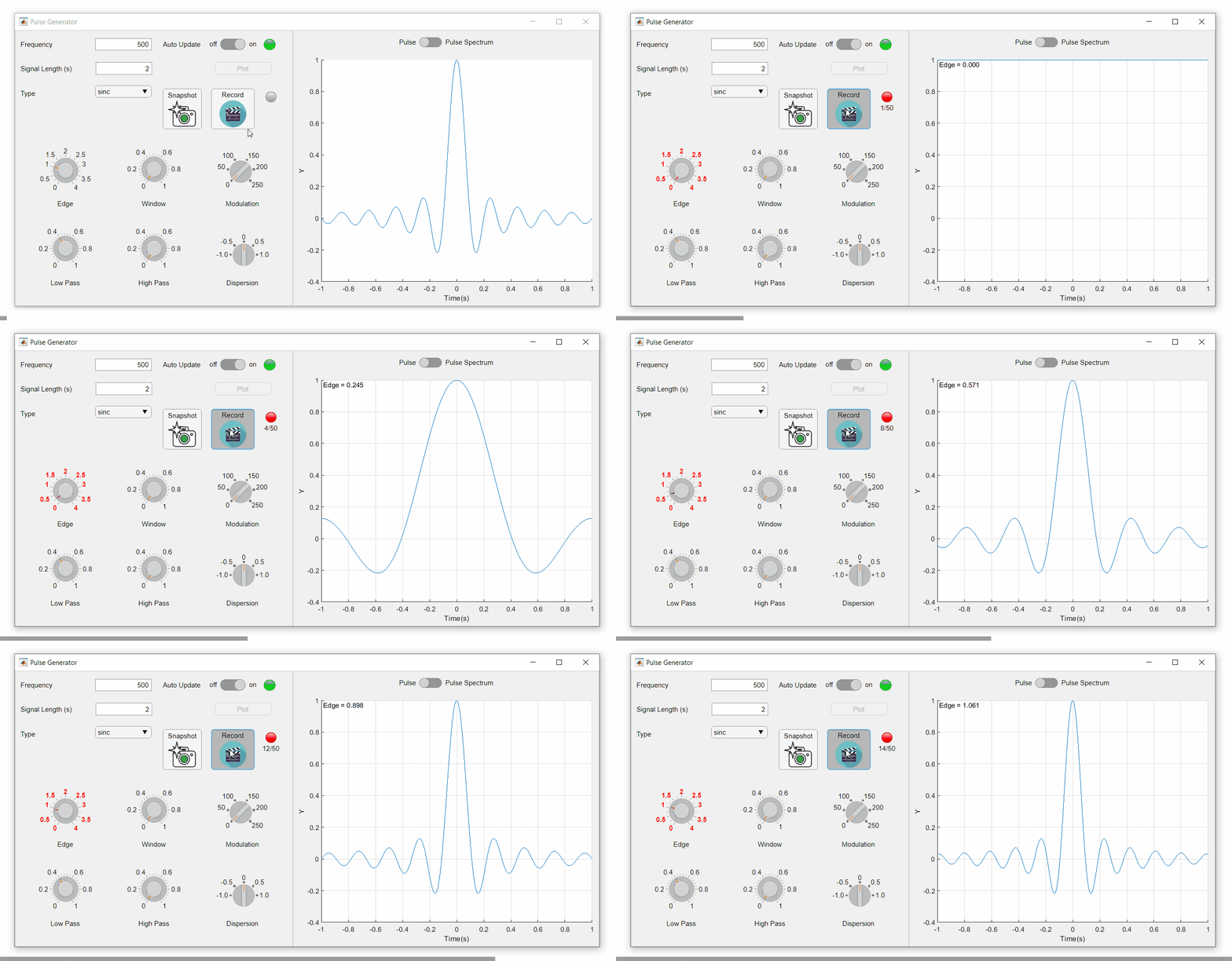
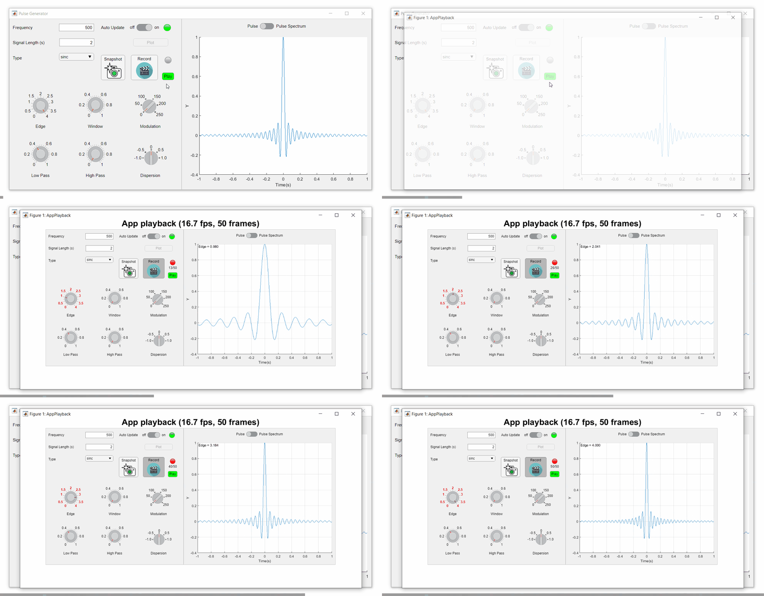
To demonstrate this, I adapted a copy of Matlab's built-in PulseGenerator.mlapp by adding
- a record button
- a record status lamp with frame counter
- a playback button
- a function that animates the effects of the Edge Knob
Recording process (The GIF is a lot faster than realtime and only shows part of the recording) (Open the image in a new window or see the attached Live Script for a clearer image).
Playback process (Open the image in a new window or see the attached Live Script for a clearer image.)
Review: How to get the handle to an app figure
To use either of these functions outside of app designer, you'll need to access the App's figure handle. By default, the HandleVisibility property of uifigures is set to off preventing the use of gcf to retrieve the figure handle. Here are 4 ways to access the app's figure handle from outside of the app.
1. Store the app's handle when opening the app.
app = myApp;
% Get the figure handle
figureHandle = app.myAppUIFigure;
2. Search for the figure handle using the app's name, tag, or any other unique property value
allfigs = findall(0, 'Type', 'figure'); % handle to all existing figures
figureHandle = findall(allfigs, 'Name', 'MyApp', 'Tag', 'MyUniqueTagName');
3. Change the HandleVisibility property to on or callback so that the figure handle is accessible by gcf anywhere or from within callback functions. This can be changed programmatically or from within the app designer component browser. Note, this is not recommended since any function that uses gcf such as axes(), clf(), etc can now access your app!.
4. If the app's figure handle is needed within a callback function external to the app, you could pass the app's figure handle in as an input variable or you could use gcbf() even if the HandleVisibility is off.
See a complete list of changes to the PulseGenerator app in the attached Live Script file to recreate the app.
File Exchange now offers the ability to download/restore previous versions of community contributed files. It's often a good practice to always update your software to the latest version, however there are times when this isn't always helpful. Sometimes a software update can break or alter something you've been relying on, in these cases you'll want to stick with the version that's working for you. This is why we've added the ability to download previous versions in File Exchange.
Using Version History
Navigate to any community member file and then click the View Version History link that appears above the Download button. This will show you a list of the previous versions contributed by the submission author. Each version will have a corresponding download button, date, version number, and a description of the changes made for that update.
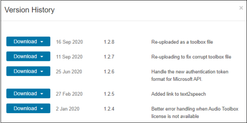
Let us know what you think about this new feature by replying below.
Here's a short article describing how educators from UNSW have used Live Scripts to help students understand mathematical models. Interactive live scripts allow students to experiment and understand concepts through trial and error. The article also explains how the scripts helped provide an enriched online learning experience for the students.
Do you use Live Scripts in your teaching?
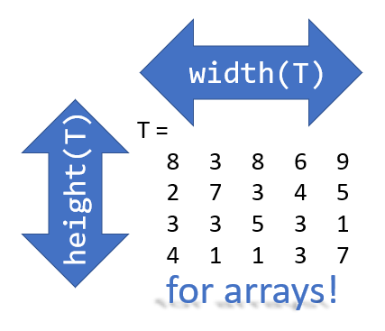
Prior to r2020b the height (number of rows) and width (number of columns) of an array or table can be determined by the size function,
array = rand(102, 16);
% Method 1
[dimensions] = size(array);
h = dimensions(1);
w = dimensions(2);
% Method 2
[h, w] = size(array); %#ok<*ASGLU>
% or
[h, ~] = size(array);
[~, w] = size(array);
% Method 3
h = size(array,1);
w = size(array,2);
In r2013b, the height(T) and width(T) functions were introduced to return the size of single dimensions for tables and timetables.
Starting in r2020b, height() and width() can be applied to arrays as an alternative to the size() function.
Continuing from the section above,
h = height(array)
% h =  102
w = width(array)
% w =  16
height() and width() can also be applied to multidimensional arrays including cell and structure arrays
mdarray = rand(4,3,20);
h = height(mdarray)
% h =  4
w = width(mdarray)
% w =  3
The expanded support of the height() and width() functions means,
- when reading code, you can no longer assume the variable T in height(T) or width(T) refers to a table or timetable
- greater flexibility in expressions such as the these, below
% C is a 1x4 cell array containing 4 matrices with different dimensions
rng('default')
C = {rand(5,2), rand(2,3), rand(3,4), rand(1,1)};
celldisp(C)
% C{1} =
%       0.81472      0.09754
%       0.90579       0.2785
%       0.12699      0.54688
%       0.91338      0.95751
%       0.63236      0.96489
% C{2} =
%       0.15761      0.95717      0.80028
%       0.97059      0.48538      0.14189
% C{3} =
%       0.42176      0.95949      0.84913      0.75774
%       0.91574      0.65574      0.93399      0.74313
%       0.79221     0.035712      0.67874      0.39223
% C{4} =
%       0.65548
What's the max number of rows in C?
maxRows1 = max(cellfun(@height,C))         % using height()
% maxRows1 =  5;
maxRows2 = max(cellfun(@(x)size(x,1),C))   % using size()
% maxRows2 =  5;
What's the total number of columns in C?
totCols1 = sum(cellfun(@width,C))          % using width()
%totCols1 =  10
totCols2 = sum(cellfun(@(x)size(x,2),C))   % using size(x,2)
% totCols2 =  10
Attached is a live script containing the content of this post.
Hi All,
Using the PMLSM SimScape block for my FOC PMLSM model - PMLSM
In the example ee_pmlsm_drive.slx which i have based my FOC architedure on, have a few questions please.
There is a gain block after the outer loop velocity controller (iq_Ref), which is the inverse of the Force constant (Kt) shown as (2/3*Np*PM) in the literature. This is also used in the PMSM FOC model, placed after the torque limiter Tq to iq_Ref. Why is this inverse Kt gain added to the idq_ref signal? Does this cancel Kt if its used in the Force Equation?
Previous help posts regarding the Force Constant (Kt), imply emitting the constant (3/2) in Kt. Also in the PMLSM help center document states Ke, Kt and Flux linkage are equal. Does this simplification apply to the translational machine counterpart SimScape block?
I have tried to look into the SimScape block code of the PMLSM to confirm, how do i look under the mask to check the Force equation for the PMLSM to confirm Kt and Ke used in this model?
Any help would be great as this is holding up Validation of my "small signal" linear PMLSM model against the SimScape PMLSM block model.
Thanks
Patrick
I'm a student. Please send me a simulation of a residential microgrid. I need this simulation for my university thesis. My thesis is about economically efficient operation of a residential microgrid using the mopso algorithm.
I often code snippets to students in the question description. I would like the students to be able to copy and paste these from the description into their solution, obviously all on the same web page. I thought this was the case before, but now Ctrl+C/V do not work and when I right click there is no copy/paste options. Is this not possible?
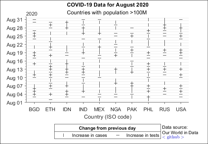
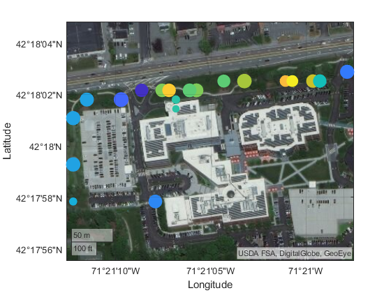
One great thing about IoT projects is they are connected to the internet, and that creates an opportunity to collaborate at a distance. Here are resources to help you teach classes that involve remote learning.

- Record and visualize your experiment's data in ThingSpeak channels. For example, this public soil monitor channel shows measurements from a sensor connected to a plant. You can see the ThingSpeak example pages for help getting your experiment connected.

- If you don’t have your own equipment see one of our 1,000,000 existing channels. Check out over 200,000 public channels at ThingSpeak.com.
- Use the fitvirus program to fit COVID-19 data. You can download the fitvirus code on File Exchange. You can get your own data or download statistics from a public ThingSpeak channel with COVID-19 data. For other COVID-19 related resources see COVID-19 Research and Development with MATLAB and Simulink

Figure 1: Fitvirus sample results.
When you can’t make it into the lab, use ThingSpeak to monitor and control your lab equipment for experiments and for teaching.
- When you use ThingSpeak channel values to control your hardware modes, students can run experiments from home, and even collaborate with others to control devices and collect data for analysis.

Figure 2: Sample ThingSpeak lab model.
- Build a simulation model to deploy on hardware and control it remotely. Watch this video to see how you can do both simulation and deployment in the same Simulink model. You can also download the models used in the video.
- Use ThingSpeak to analyze your data. Use the provided code templates (like this one for removing outliers from wind speed data) or custom MATLAB code to filter and analyze your data and schedule it to run at regular intervals.
regularFlag = isregular(data,'Time')
- Use ThingSpeak to Visualize your data. Consider a geographic plot to show location data with your measurements, or build your customized channel view.
Hi All,
Looking for guidance on how to represent a PMSM 3-Phase Converter (DC bus to AC) as a simply 1st Order Transfer Function in my Simulink model.
Researching this, have found we can show the Power Converter as a simple gain and time delay such as G_inv(s) = K_Inv/(1 + T_inv s)
The gain requires V_cm, which is the control voltage, is this control voltage the "Forward Voltage, Vf" in Switching Devices tab in the block?
Is my assumption for the tf for the converter correct?
Thanks
Patrick
Please join Loren Shure for her live sessions on the MATLAB YouTube channel starting October 1st and continuing through November 19th. You know Loren from her popular blog Loren on the Art of MATLAB.
Solve coding problems. Improve MATLAB skills. Have fun. See details and register .
I get students to create some figures in MATLAB Grader. Is there anyway the students can save the figure on their computer? I have tried savefig and that doesn't seem to do anything.
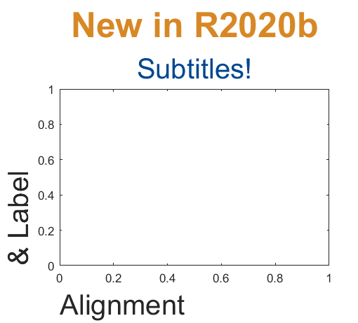
Add a subtitle
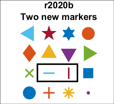
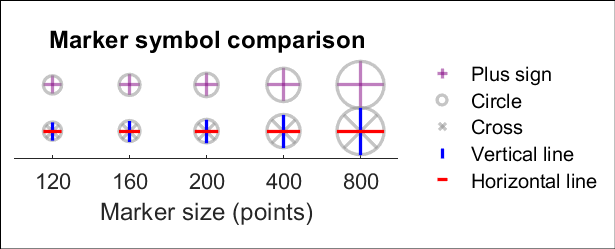
Multi-lined titles have been supported for a long time but starting in r2020b, you can add a subtitle with its own independent properties to a plot in two easy ways.
- Use the new subtitle function: s=subtitle('mySubtitle')
- Use the new second argument to the title function: [t,s]=title('myTitle','mySubtitle')
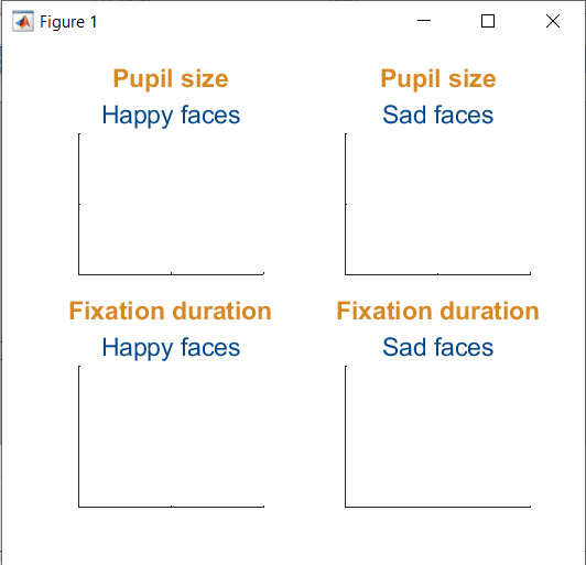
figure()
tiledlayout(2,2)
% Method 1
ax(1) = nexttile;
th(1) = title('Pupil size');
sh(1) = subtitle('Happy faces');
ax(2) = nexttile;
th(2) = title('Pupil size');
sh(2) = subtitle('Sad faces');
% Method 2
ax(3) = nexttile;
[th(3), sh(3)] = title('Fixation duration', 'Happy faces');
ax(4) = nexttile;
[th(4), sh(4)] = title('Fixation duration', 'Sad faces');
set(ax, 'xticklabel', [], 'yticklabel', [],'xlim',[0,1],'ylim',[0,1])
% Set all title colors to orange and subtitles colors to purple.
set(th, 'Color', [0.84314, 0.53333, 0.1451])
set(sh, 'Color', [0, 0.27843, 0.56078])
Control title/Label alignment
Title and axis label positions can be changed via their Position, VerticalAlignment and HorizontalAlignment properties but this is usually clumsy and leads to other problems when trying to align the title or labels with an axis edge. For example, when the position units are set to 'data' and the axis limits change, the corresponding axis label will change position relative to the axis edges. If units are normalized and the axis position or size changes, the corresponding label will no longer maintain its relative position to the axis, and that's assuming the normalized position was computed correctly in the first place.
Starting in r2020b, title and axis label alignment can be set to center|left|right, relative to the axis edges.
- TitleHorizontalAlignment is a property of the axis: h.TitleHorizontalAlignment='left';
- LabelHorizontalAlignment is a property of the ruler object that defines the x | y | z axis: h.XAxis.LabelHorizontalAlignment='left';
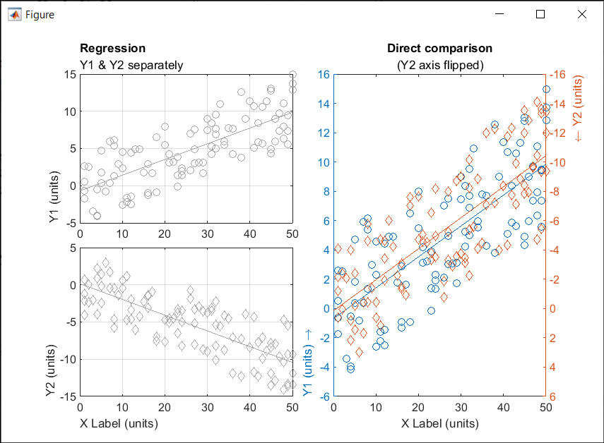
% Create data
x = randi(50,1,100)';
y = x.*[.2, -.2] + (rand(numel(x),2)-.5)*10;
gray = [.65 .65 .65];
% Plot comparison between columns of y
figure()
tiledlayout(2,2,'TileSpacing','none')
ax(1) = nexttile(1);
plot(x, y(:,1), 'o', 'color', gray)
lsline
ylabel('Y1 (units)')
title('Regression','Y1 & Y2 separately')
ax(2) = nexttile(3);
plot(x, y(:,2), 'd', 'color', gray)
lsline
xlabel('X Label (units)')
ylabel('Y2 (units)')
grid(ax, 'on')
linkaxes(ax, 'x')
%  Move title and labels leftward
set(ax, 'TitleHorizontalAlignment', 'left')
set([ax.XAxis], 'LabelHorizontalAlignment', 'left')
set([ax.YAxis], 'LabelHorizontalAlignment', 'left')
% Combine the two comparisons into plot and flip the second
% y-axis so trend are in the same direction
ax(3) = nexttile([2,1]);
yyaxis('left')
plot(x, y(:,1), 'o')
ylim([-6,16])
lsline
xlabel('X Label (units)')
ylabel('Y1 (units) \rightarrow')
yyaxis('right')
plot(x, y(:,2), 'd')
ylim([-16,6])
lsline
ylabel('\leftarrow Y2 (units)')
title('Direct comparison','(Y2 axis flipped)')
set(ax(3),  'YDir','Reverse')
% Align the ylabels with the minimum axis limit to emphasize the
% directions of each axis. Keep the title and xlabel centered
ax(3).YAxis(1).LabelHorizontalAlignment = 'left';
ax(3).YAxis(2).LabelHorizontalAlignment = 'right';
ax(3).TitleHorizontalAlignment = 'Center';       % not needed; default value.
ax(3).XAxis.LabelHorizontalAlignment = 'Center'; % not needed; default value.
Dear power electronics control community,
Since I have not solved the problem and have not found an answer to why I receive such an output, I would be happy when you could help me out. The actual project is much more extensive but easy schematic of what I want to do is here:
For that, I am using 2-level PWM generator: https://se.mathworks.com/help/physmod/sps/powersys/ref/pwmgenerator2level.html In the DC-link (DC voltage after the converter) the DC voltage output should be more-less constant (with a little noise) but right now it very far away from the desired output:
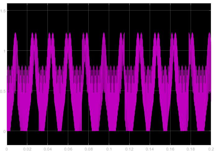
Does anyone have a idea what might cause this problem?

