Results for
Hello All,
This is my first post here so I hope its in the right place,
I have built myself a GW consisting of a RAK2245 concentrator and a Raspberry Pi, Also an Arduino end device from this link https://tum-gis-sensor-nodes.readthedocs.io/en/latest/dragino_lora_arduino_shield/README.html
Both projects work fine and connect to TTN whereby packets of data from the end device can be seen in the TTN console.
I now want to create a Webhook in TTN for Thingspeak which would hopefull allow me to see Temperature , Humidity etc in graphical form.
My question, does thingspeak support homebuilt devices or is it focused on comercially built devices ?
I have spent many hours trying to find data hosting site that is comepletely free for a few devices and not to complicated to setup as some seem to be a nightmare. Thanks for any support .
At #9 in our MATLAB EXPO 2025 countdown: From Tinkerer to Developer—A Journey in Modern Engineering Software Development
A big thank‑you to Greg Diehl at NAVAIR and Michelle Allard at MathWorks, the team behind this session, for sharing their multi‑year evolution from rapid‑fire experimenting to disciplined, scalable software development.
If you’ve ever wondered what it really takes to move MATLAB code from “it works!” to “it’s ready for production,” this talk captures that transition. The team highlights how improved testing practices, better structure, and close collaboration with MathWorks experts helped them mature their workflows and tackle challenges around maintainability and code quality.
Curious about the pivotal moments that helped them level up their engineering software practices?
How can I found my license I'd and password, so please provide me my id
Over the past few days I noticed a minor change on the MATLAB File Exchange:
For a FEX repository, if you click the 'Files' tab you now get a file-tree–style online manager layout with an 'Open in new tab' hyperlink near the top-left. This is very useful:
If you want to share that specific page externally (e.g., on GitHub), you can simply copy that hyperlink. For .mlx files it provides a perfect preview. I'd love to hear your thoughts.
EXAMPLE:
🤗🤗🤗
I wanted to share something I've been thinking about to get your reactions. We all know that most MATLAB users are engineers and scientists, using MATLAB to do engineering and science. Of course, some users are professional software developers who build professional software with MATLAB - either MATLAB-based tools for engineers and scientists, or production software with MATLAB Coder, MATLAB Compiler, or MATLAB Web App Server.
I've spent years puzzling about the very large grey area in between - engineers and scientists who build useful-enough stuff in MATLAB that they want their code to work tomorrow, on somebody else's machine, or maybe for a large number of users. My colleagues and I have taken to calling them "Reluctant Developers". I say "them", but I am 1,000% a reluctant developer.
I first hit this problem while working on my Mech Eng Ph.D. in the late 90s. I built some elaborate MATLAB-based tools to run experiments and analysis in our lab. Several of us relied on them day in and day out. I don't think I was out in the real world for more than a month before my advisor pinged me because my software stopped working. And so began a career of building amazing, useful, and wildly unreliable tools for other MATLAB users.
About a decade ago I noticed that people kept trying to nudge me along - "you should really write tests", "why aren't you using source control". I ignored them. These are things software developers do, and I'm an engineer.
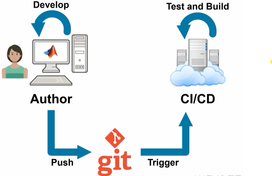
I think it finally clicked for me when I listened to a talk at a MATLAB Expo around 2017. An aerospace engineer gave a talk on how his team had adopted git-based workflows for developing flight control algorithms. An attendee asked "how do you have time to do engineering with all this extra time spent using software development tools like git"? The response was something to the effect of "oh, we actually have more time to do engineering. We've eliminated all of the waste from our unamanaged processes, like multiple people making similar updates or losing track of the best version of an algorithm." I still didn't adopt better practices, but at least I started to get a sense of why I might.
Fast-forward to today. I know lots of users who've picked up software dev tools like they are no big deal, but I know lots more who are still holding onto their ad-hoc workflows as long as they can. I'm on a bit of a campaign to try to change this. I'd like to help MATLAB users recognize when they have problems that are best solved by borrowing tools from our software developer friends, and then give a gentle onramp to using these tools with MATLAB.
I recently published this guide as a start:
Waddya think? Does the idea of Reluctant Developer resonate with you? If you take some time to read the guide, I'd love comments here or give suggestions by creating Issues on the guide on GitHub (there I go, sneaking in some software dev stuff ...)
Couldn’t catch everything at MATLAB EXPO 2025? You’re not alone. Across keynotes and track talks, there were too many gems for one sitting. For the next 9 weeks, we’ll reveal the "Top 10" sessions attended (workshops excluded)—one per week—so you can binge the best and compare notes with peers.
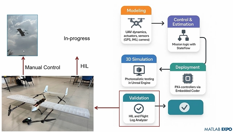
Starting at #10: Simulation-Driven Development of Autonomous UAVs Using MATLAB
A huge thanks to Dr. Shital S. Chiddarwar from Visvesvaraya National Institute of Technology Nagpur who delivered this presentation online at MATLAB EXPO 2025. Are you curious how this workflow accelerates development and boosts reliability?
I recently created a short 5-minute video covering 10 tips for students learning MATLAB. I hope this helps!
DocMaker allows you to create MATLAB toolbox documentation from Markdown documents and MATLAB scripts.
The MathWorks Consulting group have been using it for a while now, and so David Sampson, the director of Application Engineering, felt that it was time to share it with the MATLAB and Simulink community.
David listed its features as:
➡️ write documentation in Markdown not HTML
🏃 run MATLAB code and insert textual and graphical output
📜 no more hand writing XML index files
🕸️ generate documentation for any release from R2021a onwards
💻 view and edit documentation in MATLAB, VS Code, GitHub, GitLab, ...
🎉 automate toolbox documentation generation using MATLAB build tool
📃 fully documented using itself
😎 supports light, dark, and responsive modes
🐣 cute logo
I got an email message that says all the files I've uploaded to the File Exchange will be given unique names. Are these new names being applied to my files automatically? If so, do I need to download them to get versions with the new name so that if I update them they'll have the new name instead of the name I'm using now?
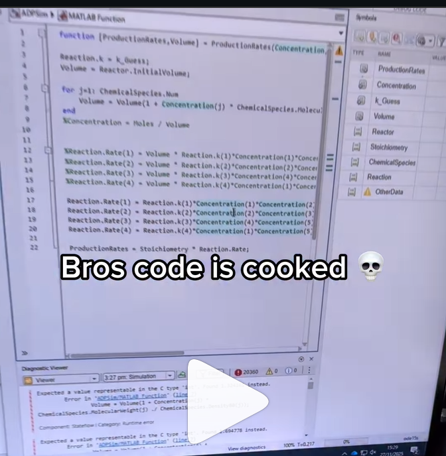
A coworker shared with me a hilarious Instagram post today. A brave bro posted a short video showing his MATLAB code… casually throwing 49,000 errors!
Surprisingly, the video went virial and recieved 250,000+ likes and 800+ comments. You really never know what the Instagram algorithm is thinking, but apparently “my code is absolutely cooked” is a universal developer experience 😂
Last note: Can someone please help this Bro fix his code?
Is it possible to display a variable value within the ThingSpeak plot area?
https://www.mathworks.com/matlabcentral/answers/2182045-why-can-t-i-renew-or-purchase-add-ons-for-m…
"As of January 1, 2026, Perpetual Student and Home offerings have been sunset and replaced with new Annual Subscription Student and Home offerings."
So, Perpetual licenses for Student and Home versions are no more. Also, the ability for Student and Home to license just MATLAB by itself has been removed.
The new offering for Students is $US119 per year with no possibility of renewing through a Software Maintenance Service type offering. That $US119 covers the Student Suite of MATLAB and Simulink and 11 other toolboxes. Before, the perpetual license was $US99... and was a perpetual license, so if (for example) you bought it in second year you could use it in third and fourth year for no additional cost. $US99 once, or $US99 + $US35*2 = $US169 (if you took SMS for 2 years) has now been replaced by $US119 * 3 = $US357 (assuming 3 years use.)
The new offering for Home is $US165 per year for the Suite (MATLAB + 12 common toolboxes.) This is a less expensive than the previous $US150 + $US49 per toolbox if you had a use for those toolboxes . Except the previous price was a perpetual license. It seems to me to be more likely that Home users would have a use for the license for extended periods, compared to the Student license (Student licenses were perpetual licenses but were only valid while you were enrolled in degree granting instituations.)
Unfortunately, I do not presently recall the (former) price for SMS for the Home license. It might be the case that by the time you added up SMS for base MATLAB and the 12 toolboxes, that you were pretty much approaching $US165 per year anyhow... if you needed those toolboxes and were willing to pay for SMS.
But any way you look at it, the price for the Student version has effectively gone way up. I think this is a bad move, that will discourage students from purchasing MATLAB in any given year, unless they need it for courses. No (well, not much) more students buying MATLAB with the intent to explore it, knowing that it would still be available to them when it came time for their courses.
You may have come across code that looks like that in some languages:
stubFor(get(urlPathEqualTo("/quotes"))
.withHeader("Accept", equalTo("application/json"))
.withQueryParam("s", equalTo(monitoredStock))
.willReturn(aResponse())
.withStatus(200)
.withHeader("Content-Type", "application/json")
.withBody("{\\"symbol\\": \\"XYZ\\", \\"bid\\": 20.2, " + "\\"ask\\": 20.6}")))
That’s Java. Even if you can’t fully decipher it, you can get a rough idea of what it is supposed to do, build a rather complex API query.
Or you may be familiar with the following similar and frequent syntax in Python:
import seaborn as sns
sns.load_dataset('tips').sample(10, random_state=42).groupby('day').mean()
Here’s is how it works: multiple method calls are linked together in a single statement, spanning over one or several lines, usually because each method returns the same object or another object that supports further calls.
That technique is called method chaining and is popular in Object-Oriented Programming.
A few years ago, I looked for a way to write code like that in MATLAB too. And the answer is that it can be done in MATLAB as well, whevener you write your own class!
Implementing a method that can be chained is simply a matter of writing a method that returns the object itself.
In this article, I would like to show how to do it and what we can gain from such a syntax.
Example
A few years ago, I first sought how to implement that technique for a simulation launcher that had lots of parameters (far too many):
lauchSimulation(2014:2020, true, 'template', 'TmplProd', 'Priority', '+1', 'Memory', '+6000')
As you can see, that function takes 2 required inputs, and 3 named parameters (whose names aren’t even consistent, with ‘Priority’ and ‘Memory’ starting with an uppercase letter when ‘template’ doesn’t).
(The original function had many more parameters that I omit for the sake of brevity. You may also know of such functions in your own code that take a dozen parameters which you can remember the exact order.)
I thought it would be nice to replace that with:
SimulationLauncher() ...
.onYears(2014:2020) ...
.onDistributedCluster() ... % = equivalent of the previous "true"
.withTemplate('TmplProd') ...
.withPriority('+1') ...
.withReservedMemory('+6000') ...
.launch();
The first 6 lines create an object of class SimulationLauncher, calls several methods on that object to set the parameters, and lastly the method launch() is called, when all desired parameters have been set.
To make it cleared, the syntax previously shown could also be rewritten as:
launcher = SimulationLauncher();
launcher = launcher.onYears(2014:2020);
launcher = launcher.onDistributedCluster();
launcher = launcher.withTemplate('TmplProd');
launcher = launcher.withPriority('+1');
launcher = launcher.withReservedMemory('+6000');
launcher.launch();
Before we dive into how to implement that code, let’s examine the advantages and drawbacks of that syntax.
Benefits and drawbacks
Because I have extended the chained methods over several lines, it makes it easier to comment out or uncomment any one desired option, should the need arise. Furthermore, we need not bother any more with the order in which we set the parameters, whereas the usual syntax required that we memorize or check the documentation carefully for the order of the inputs.
More generally, chaining methods has the following benefits and a few drawbacks:
Benefits:
- Conciseness: Code becomes shorter and easier to write, by reducing visual noise compared to repeating the object name.
- Readability: Chained methods create a fluent, human-readable structure that makes intent clear.
- Reduced Temporary Variables: There's no need to create intermediary variables, as the methods directly operate on the object.
Drawbacks:
- Debugging Difficulty: If one method in a chain fails, it can be harder to isolate the issue. It effectively prevents setting breakpoints, inspecting intermediate values, and identifying which method failed.
- Readability Issues: Overly long and dense method chains can become hard to follow, reducing clarity.
- Side Effects: Methods that modify objects in place can lead to unintended side effects when used in long chains.
Implementation
In the SimulationLauncher class, the method lauch performs the main operation, while the other methods just serve as parameter setters. They take the object as input and return the object itself, after modifying it, so that other methods can be chained.
classdef SimulationLauncher
properties (GetAccess = private, SetAccess = private)
years_
isDistributed_ = false;
template_ = 'TestTemplate';
priority_ = '+2';
memory_ = '+5000';
end
methods
function varargout = launch(obj)
% perform whatever needs to be launched
% using the values of the properties stored in the object:
% obj.years_
% obj.template_
% etc.
end
function obj = onYears(obj, years)
assert(isnumeric(years))
obj.years_ = years;
end
function obj = onDistributedCluster(obj)
obj.isDistributed_ = true;
end
function obj = withTemplate(obj, template)
obj.template_ = template;
end
function obj = withPriority(obj, priority)
obj.priority_ = priority;
end
function obj = withMemory( obj, memory)
obj.memory_ = memory;
end
end
end
As you can see, each method can be in charge of verifying the correctness of its input, independantly. And what they do is just store the value of parameter inside the object. The class can define default values in the properties block.
You can configure different launchers from the same initial object, such as:
launcher = SimulationLauncher();
launcher = launcher.onYears(2014:2020);
launcher1 = launcher ...
.onDistributedCluster() ...
.withReservedMemory('+6000');
launcher2 = launcher ...
.withTemplate('TmplProd') ...
.withPriority('+1') ...
.withReservedMemory('+7000');
If you call the same method several times, only the last recorded value of the parameter will be taken into acount:
launcher = SimulationLauncher();
launcher = launcher ...
.withReservedMemory('+6000') ...
.onDistributedCluster() ...
.onYears(2014:2020) ...
.withReservedMemory('+7000') ...
.withReservedMemory('+8000');
% The value of "memory" will be '+8000'.
If the logic is still not clear to you, I advise you play a bit with the debugger to better understand what’s going on!
Conclusion
I love how the method chaining technique hides the minute detail that we don’t want to bother with when trying to understand what a piece of code does.
I hope this simple example has shown you how to apply it to write and organise your code in a more readable and convenient way.
Let me know if you have other questions, comments or suggestions. I may post other examples of that technique for other useful uses that I encountered in my experience.
I’m currently developing a multi-platform viewer using Flutter to eliminate the hassle of manual channel setup. Instead of adding IDs one by one, the app uses your User API Key to automatically discover and list all your ThingSpeak channels instantly.
Key Highlights (Work in Progress):
- Automatic Sync: All your channels appear in seconds.
- Multi-platform: Built for Web, Android, Windows, and Linux.
- Privacy-Focused: Secure local storage for your API keys.
If you use tables extensively to perform data analysis, you may at some point have wanted to add new functionalities suited to your specific applications. One straightforward idea is to create a new class that subclasses the built-in table class. You would then benefit from all inherited existing methods.
One workaround is to create a new class that wraps a table as a Property, and re-implement all the methods that you need and are already defined for table. The is not too difficult, except for the subsref method, for which I’ll provide the code below.
Class definition
Defining a wrapper of the table class is quite straightforward. In this example, I call the class “Report” because that is what I intend to use the class for, to compute and store reports. The constructor just takes a table as input:
classdef Rapport
methods
function obj = Report(t)
if isa(t, 'Report')
obj = t;
else
obj.t_ = t;
end
end
end
properties (GetAccess = private, SetAccess = private)
t_ table = table();
end
end
I designed the constructor so that it converts a table into a Report object, but also so that if we accidentally provide it with a Report object instead of a table, it will not generate an error.
Reproducing the behaviour of the table class
Implementing the existing methods of the table class for the Report class if pretty easy in most cases.
I made use of a method called “table” in order to be able to get the data back in table format instead of a Report, instead of accessing the property t_ of the object. That method can also be useful whenever you wish to use the methods or functions already existing for tables (such as writetable, rowfun, groupsummary…).
classdef Rapport
...
methods
function t = table(obj)
t = obj.t_;
end
function r = eq(obj1,obj2)
r = isequaln(table(obj1), table(obj2));
end
function ind = size(obj, varargin)
ind = size(table(obj), varargin{:});
end
function ind = height(obj, varargin)
ind = height(table(obj), varargin{:});
end
function ind = width(obj, varargin)
ind = width(table(obj), varargin{:});
end
function ind = end(A,k,n)
% ind = end(A.t_,k,n);
sz = size(table(A));
if k < n
ind = sz(k);
else
ind = prod(sz(k:end));
end
end
end
end
In the case of horzcat (same principle for vertcat), it is just a matter of converting back and forth between the table and Report classes:
classdef Rapport
...
methods
function r = horzcat(obj1,varargin)
listT = cell(1, nargin);
listT{1} = table(obj1);
for k = 1:numel(varargin)
kth = varargin{k};
if isa(kth, 'Report')
listT{k+1} = table(kth);
elseif isa(kth, 'table')
listT{k+1} = kth;
else
error('Input must be a table or a Report');
end
end
res = horzcat(listT{:});
r = Report(res);
end
end
end
Adding a new method
The plus operator already exists for the table class and works when the table contains all numeric values. It sums columns as long as the tables have the same length.
Something I think would be nice would be to be able to write t1 + t2, and that would perform an outerjoin operation between the tables and any sizes having similar indexing columns.
That would be so concise, and that's what we’re going to implement for the Report class as an example. That is called “plus operator overloading”. Of course, you could imagine that the “+” operator is used to compute something else, for example adding columns together with regard to the keys index. That depends on your needs.
Here’s a unittest example:
classdef ReportTest < matlab.unittest.TestCase
methods (Test)
function testPlusOperatorOverload(testCase)
t1 = array2table( ...
{ 'Smith', 'Male' ...
; 'JACKSON', 'Male' ...
; 'Williams', 'Female' ...
} , 'VariableNames', {'LastName' 'Gender'} ...
);
t2 = array2table( ...
{ 'Smith', 13 ...
; 'Williams', 6 ...
; 'JACKSON', 4 ...
}, 'VariableNames', {'LastName' 'Age'} ...
);
r1 = Report(t1);
r2 = Report(t2);
tRes = r1 + r2;
tExpected = Report( array2table( ...
{ 'JACKSON' , 'Male', 4 ...
; 'Smith' , 'Male', 13 ...
; 'Williams', 'Female', 6 ...
} , 'VariableNames', {'LastName' 'Gender' 'Age'} ...
) );
testCase.verifyEqual(tRes, tExpected);
end
end
end
And here’s how I’d implement the plus operator in the Report class definition, so that it also works if I add a table and a Report:
classdef Rapport
...
methods
function r = plus(obj1,obj2)
table1 = table(obj1);
table2 = table(obj2);
result = outerjoin(table1, table2 ...
, 'Type', 'full', 'MergeKeys', true);
r = reportingits.dom.Rapport(result);
end
end
end
The case of the subsref method
If we wish to access the elements of an instance the same way we would with regular tables, whether with parentheses, curly braces or directly with the name of the column, we need to implement the subsref and subsasgn methods. The second one, subsasgn is pretty easy, but subsref is a bit tricky, because we need to detect whether we’re directing towards existing methods or not.
Here’s the code:
classdef Rapport
...
methods
function A = subsasgn(A,S,B)
A.t_ = subsasgn(A.t_,S,B);
end
function B = subsref(A,S)
isTableMethod = @(m) ismember(m, methods('table'));
isReportMethod = @(m) ismember(m, methods('Report'));
switch true
case strcmp(S(1).type, '.') && isReportMethod(S(1).subs)
methodName = S(1).subs;
B = A.(methodName)(S(2).subs{:});
if numel(S) > 2
B = subsref(B, S(3:end));
end
case strcmp(S(1).type, '.') && isTableMethod (S(1).subs)
methodName = S(1).subs;
if ~isReportMethod(methodName)
error('The method "%s" needs to be implemented!', methodName)
end
otherwise
B = subsref(table(A),S(1));
if istable(B)
B = Report(B);
end
if numel(S) > 1
B = subsref(B, S(2:end));
end
end
end
end
end
Conclusion
I believe that the table class is Sealed because is case new methods are introduced in MATLAB in the future, the subclass might not be compatible if we created any or generate unexpected complexity.
The table class is a really powerful feature.
I hope this example has shown you how it is possible to extend the use of tables by adding new functionalities and maybe given you some ideas to simplify some usages. I’ve only happened to find it useful in very restricted cases, but was still happy to be able to do so.
In case you need to add other methods of the table class, you can see the list simply by calling methods(’table’).
Feel free to share your thoughts or any questions you might have! Maybe you’ll decide that doing so is a bad idea in the end and opt for another solution.
Missed a session or want to revisit your favorites? Now’s your chance!
Explore 42 sessions packed with insights, including:
✅4 inspiring keynotes
✅ 22 Customer success stories
✅5 Partner innovations
✅11 MathWorks-led technical talks
Each session comes with video recordings and downloadable slides, so you can learn at your own pace.
I can't believe someone put time into this ;-)

Our exportgraphics and copygraphics functions now offer direct and intuitive control over the size, padding, and aspect ratio of your exported figures.
- Specify Output Size: Use the new Width, Height, and Units name-value pairs
- Control Padding: Easily adjust the space around your axes using the Padding argument, or set it to to match the onscreen appearance.
- Preserve Aspect Ratio: Use PreserveAspectRatio='on' to maintain the original plot proportions when specifying a fixed size.
- SVG Export: The exportgraphics function now supports exporting to the SVG file format.
Check out the full article on the Graphics and App Building blog for examples and details: Advanced Control of Size and Layout of Exported Graphics
No, staying home (or where I'm now)
25%
Yes, 1 night
0%
Yes, 2 nights
12.5%
Yes, 3 nights
12.5%
Yes, 4-7 nights
25%
Yes, 8 nights or more
25%
8 votes
Hi everyone
I've been using ThingSpeak for several years now without an issue until last Thursday.
I have four ThingSpeak channels which are used by three Arduino devices (in two locations/on two distinct networks) all running the same code.
All three devices stopped being able to write data to my ThingSpeak channels around 17:00 CET on 4 Dec and are still unable to.
Nothing changed on this side, let alone something that would explain the problem.
I would note that data can still be written to all the channels via a browser so there is no fundamental problem with the channels (such as being full).
Since the above date and time, any HTTP/1.1 'update' (write) requests via the REST API (using both simple one-write GET requests or bulk JSON POST requests) are timing out after 5 seconds and no data is being written. The 5 second timeout is my Arduino code's default, but even increasing it to 30 seconds makes no difference. Before all this, responses from ThingSpeak were sub-second.
I have recompiled the Arduino code using the latest libraries and that didn't help.
I have tested the same code again another random api (api.ipify.org) and that works just fine.
Curl works just fine too, also usng HTTP/1.1
So the issue appears to be something particular to the combination of my Arduino code *and* the ThingSpeak environment, where something changed on the ThingSpeak end at the above date and time.
If anyone in the community has any suggestions as to what might be going on, I would greatly appreciate the help.
Peter