Results for
I spent some time tonight updating the UIHTML App skills on the MATLAB Agent Skills Playground hosted on GitHub.
We are using this repo to share early ideas and experiments with agent skills.
When you are trying to bring the latest update into a coding like Codex, you can point the agent at a secret file called "llms.txt" -- this is file optimized for coding agents. I use it to over come "training data" bias. As even the latest models have outdated doc. This is important for working with projects that up date frequently.
Here are some of my favorites to use:
n= input('Escolhe um número inteiro postivo. ')
primo=true;
i=2;
while i<n
if mod(n,i)==0;
primo=false;
end
i= i+1;
end
if primo && n>1;
disp('É primo')
else
disp('Não é primo')
end
anterior= n-1;
while true
primo=true;
i=2;
while i< anterior
if mod(anterior,i)==0;
primo= false;
end
i= i+1;
end
if primo && anterior>1;
end
anterior= anterior-1;
end
disp(anterior)
seguinte= n+1;
while true;
primo= true;
i=2;
while i<seguinte;
if mod(seguinte,i)==0;
primo=false;
end
i=i+1;
end
if primo && seguinte>1;
end
seguinte= seguinte+1;
end
disp(seguinte)
Any ideas? It is in portuguese if you intend to translate it.
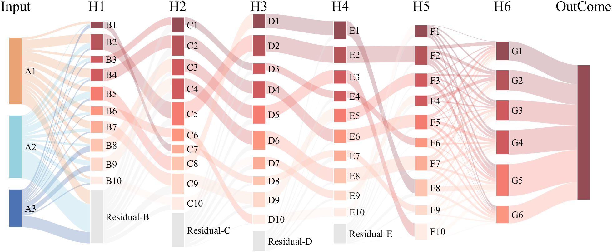
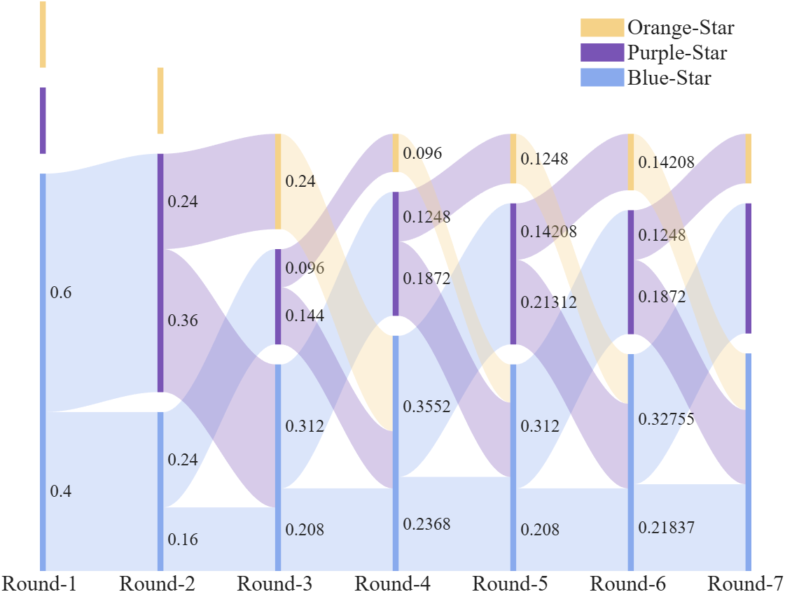
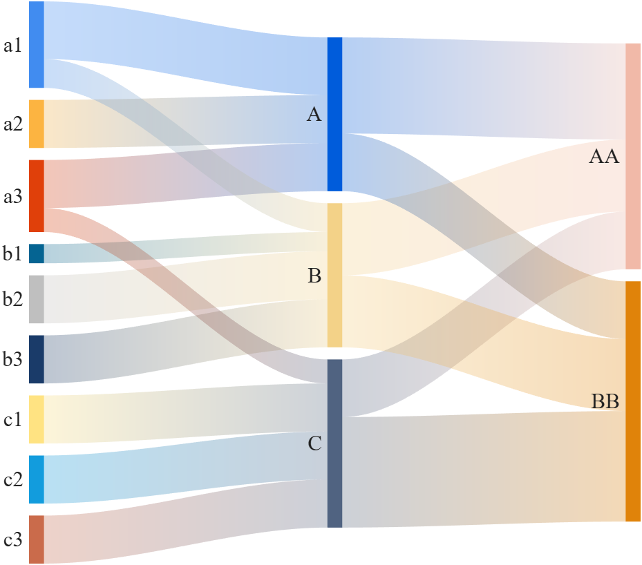
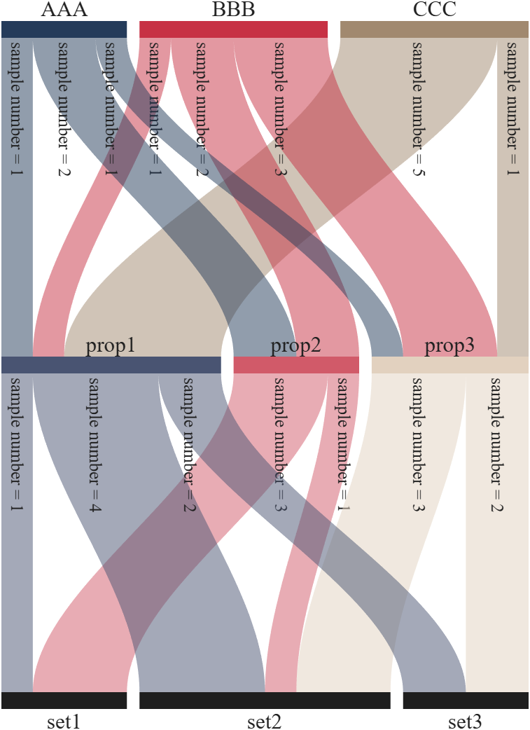
This is a brief introduction and recommendation of a Sankey diagram plotting tool:
Basic usage - links
links={'a1','A',1.2;'a2','A',1;'a1','B',.6;'a3','A',1; 'a3','C',0.5;
'b1','B',.4; 'b2','B',1;'b3','B',1; 'c1','C',1;
'c2','C',1; 'c3','C',1;'A','AA',2; 'A','BB',1.2;
'B','BB',1.5; 'B','AA',1.5; 'C','BB',2.3; 'C','AA',1.2};
% 创建桑基图对象(Create a Sankey diagram object)
SK=SSankey(links(:,1),links(:,2),links(:,3));
% 开始绘图(Start drawing)
SK.draw()
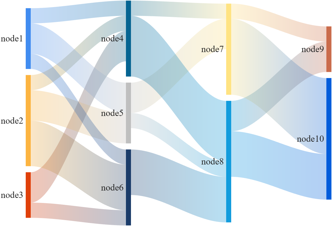
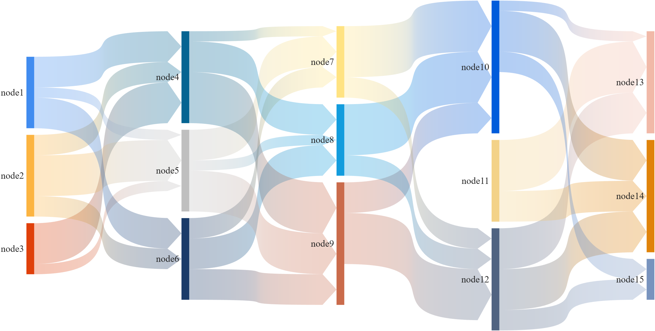
Basic usage - adjMat
% Define inter-layer adjacency matrices
% 定义层间邻接矩阵
A12 = [1,2,1; 1,2,3; 2,0,1];
A23 = [1,4; 2,1; 0,3];
A34 = [1,5; 2,3];
% Assemble global block matrix (main diagonal = zero, super-diagonal = A12, A23, A34)
% 组装全局分块矩阵(主对角线为零,上对角线为 A12, A23, A34)
adjMat = mergeAdjMat({A12, A23, A34});
SK = SSankey([],[],[], 'AdjMat',adjMat);
SK.draw()
Further usage examples can be found in the demos included in the compressed package:
MATLAB AI Agent SDK lets you build and run AI agents in MATLAB.
- Create agents based on OpenAI®, Ollama™, or OpenAI-compatible APIs.
- Integrate LLMs and agentic workflows into your workflows in a targeted manner, retaining deterministic workflows when those are more suitable.
- Let your agent work on large amounts of data without needing to send the data to the LLM.
This SDK is a Research Preview under active development and APIs may change.
How much faster does a small GPT train on an Apple Silicon GPU?
Duncan Carlsmith, Department of Physics, University of Wisconsin-Madison
Introduction
My prior post nanoGPT Arithmetic Explorer: A small MATLAB GPT that groks integer addition, and my FEX submission nanoGPT Arithmetic Explorer present a small character-level GPT in MATLAB that learns integer addition, trained entirely on the CPU. That project raised for me a practical question for anyone who, like me, runs MATLAB on a Mac: MATLAB has no GPU support on Apple Silicon - gpuArray and the Deep Learning Toolbox training path require an NVIDIA CUDA GPU - yet every M-series Mac carries a capable GPU, arguably a built-in NVIDIA Spark equivalent, that sits idle while the model trains. APPLE GPUs have reduced precision, but that is perhaps not relevant, even valued, in GPT applications. To access the APPLE GPU requires indirect methods. My new Live Script Mac GPT GPU Benchmark Explorer explores the speed up for small models with a small, reproducible GPT benchmark for any Mac.
The workload is the same small GPT learning addition, so each variant can be checked to actually learn - to grok perfect answers on held-out problems. The same model is trained three ways on the same machine: the original MATLAB engine on the CPU, PyTorch on the CPU, and PyTorch on the Metal GPU through Apple's MPS backend. Three points let the total speedup factor into a framework effect and a device effect. The nanoGPT model is flexible in size, allowing extrapolation to larger models not needed in the arithmetic application.
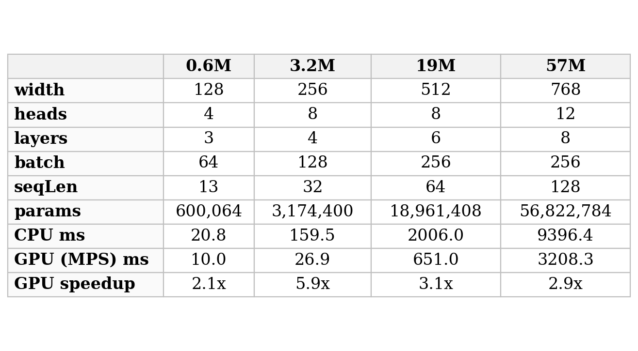
On my M1 Max, the result is about a 7.7x speedup per training step moving from the MATLAB workflow to PyTorch on the GPU, and it factors as roughly 3.7x from the framework times 2.1x from the device. Most of the gain is not the GPU: likely PyTorch's fused attention, tuned linear algebra, and lighter automatic differentiation account for the larger factor, and the Metal GPU roughly doubles it again. With a fixed model seed, the CPU and GPU loss curves agree to several decimals, and both grok to perfect accuracy, so this is the same computation, only faster - all in single precision, which is what neural-network training often uses anyway and what every Apple GPU provides.
The script also pits Apple's own MLX framework against PyTorch on the GPU. MLX has its own Metal kernels and edges, PyTorch only for the smallest models; PyTorch pulls ahead as the model grows. A size sweep shows the GPU advantage ranging from roughly two to six times across a wide range of model sizes. Caveats: a laptop throttles under sustained load, so a long run reads slower per step than a short, timed burst. Other factors may enter. I'm no expert in benchmarking practices.
Table 1. The size sweep on the reference machine (Apple M1 Max): each column is one model configuration, headed by its parameter count, with the per-step training time on the CPU and on the Apple GPU (PyTorch-MPS). GPU speedup is CPU time divided by GPU time. It is a compound sweep - width, heads, layers, batch, and sequence length all change together.
 The Live Script is organized as three panels - the three-point comparison, the speedup-versus-size sweep, and the MLX-versus-PyTorch contrast. Each panel displays a precomputed result shipped with the package by default, and each has a "Try this" switch that regenerates it on your own Mac. A set of challenges suggests the reader extend the study, for example, with controlled single-variable sweeps or a run on a different Apple chip. The self-contained arithGPT trainer is bundled with the script; the GPU work runs in PyTorch and MLX, both free and open-source, with no paid API. The package and this writeup were built with Claude (Anthropic) working with MATLAB R2026a on my own MacBook with an M1 chip through an ngrok command server, the agentic context described in my prior posts.
A note on hardware: what "capable" means
Three numbers describe a GPU for this kind of work. Compute is measured in TFLOPS - trillions of floating-point arithmetic operations per second - quoted at a stated numeric precision; FP32 means 32-bit floating-point numbers, the full-precision arithmetic this article trains in, and the standard for scientific computing. Memory bandwidth, in gigabytes per second (GB/s), is how fast the chip moves data between memory and its arithmetic units; for the small models trained here, that is often the real limit, rather than raw compute. Unified memory, in gigabytes (GB), is the single pool of memory that the CPU and GPU share on these chips, which sets how large a model can be held at once. The last row of the table is simply whether MATLAB's own GPU functions (gpuArray, trainnet) run on the machine: they require NVIDIA's CUDA platform, which no Apple Silicon Mac provides.
Table 2. GPU capability of the M1 Max used in this study, Apple's current M5 and M5 Max, and NVIDIA's DGX Spark, all at FP32 precision. Higher TFLOPS and bandwidth are faster; unified memory sets the largest model that fits; the last row is whether MATLAB's built-in GPU training runs on the machine.
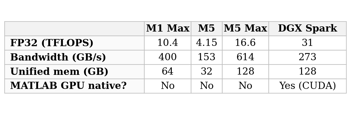
The M1 Max used here delivers about 10 TFLOPS of FP32 at 400 GB/s - genuinely capable, and in fact more memory bandwidth than the brand-new DGX Spark. Apple's current line runs from the small M5 (4.15 TFLOPS, lower than the older M1 Max because it is the entry-level chip) up to the M5 Max (16.6 TFLOPS, 614 GB/s, 128 GB), the true successor that beats the M1 Max on every count.
The DGX Spark plays a different game. Its FP32 figure of about 31 TFLOPS is only part of the story; its real strength is arithmetic at very low precision, which Apple's GPUs do not offer. NVIDIA's headline 'one petaFLOP' (a thousand TFLOPS) is an FP4 number - 4-bit floating-point, sixteen times coarser than FP32 - and it also counts sparsity, a hardware trick that skips multiplications by zero; without that trick, it is about half as much. Four-bit numbers are far too coarse to train with, but they are precise enough to run an already-trained very large model, which is what the Spark is built for: large-model use on the desktop, not the full-precision training measured here. The detail that matters for this article is the last table row - because the Spark runs CUDA on Linux, MATLAB's own GPU training path works on it directly, the very thing that does not exist on any Mac, and the reason this study reached for PyTorch and MLX.
References
Duncan Carlsmith (2026). Mac GPT GPU Benchmark Explorer (https://www.mathworks.com/matlabcentral/fileexchange/184058-mac-gpt-gpu-benchmark-explorer), MATLAB Central File Exchange. Retrieved June 12, 2026.
Acknowledgements
This submission and the FEX submission build and test were made with the assistance of Anthropic Claude in a few hours. The author has relied heavily on Claude's expertise. Caveat emptor.
Conflict of interest
The author declares he has no financial interest in MathWorks, Anthropic, or Apple. This article is informational and does not constitute an endorsement by the University of Wisconsin-Madison of any vendor or product. Claude is a trademark of Anthropic. MATLAB is a trademark of MathWorks. PyTorch, MLX, and Metal are trademarks of their respective owners.
 A small MATLAB GPT that groks integer addition
Duncan Carlsmith, Department of Physics, University of Wisconsin-Madison
Introduction
My prior post A miniature GPT language model as a MATLAB Live Script provides a small character-level GPT in MATLAB and trains it on Shakespeare. Language modeling is intractable in the sense that there is no exact answer to grade against; the model is judged by whether its output reads plausibly. This companion Live Script applies the same architecture to a problem with a clear success metric. The goal of training is for the model to discover/get/“grok” an exact algorithm for integer addition in any base (e.g., binary, decimal, and hexadecimal). With this script, you can watch a “grok,” the model suddenly “getting” addition, happen in real time and in detail- very fun if you are like me, hardly an expert!
Addition is easy except for the carry. The digit in a column is the column sum modulo the base. The carry couples columns: a carry out of one column feeds the next, and consecutive carries chain groups of columns together. The script grades the model on held-out problems sorted by the length of the longest carry chain, so the per-chain accuracy curves show exactly where and how the model succeeds. One observes the model first grok single carries, then singles and doubles, and so on, up to the maximum for the range of digits presented during training. In representing a finite range of numbers, the distribution of carry chain lengths depends on the base, as does the number of essential tokens. Hence, although the essence of addition is base-independent, the learning curves are different for different bases.
As is well known, the grok duration can be very short or gradual, depending on exactly how the addition problem is posed when presented to the model and if a random or structured learning curriculum is used. The script demonstrates that since a random number generator based on a seed is used to generate training samples, the time and even existence of a grok in a prescribed length set of training steps fluctuates, sometimes wildly, but for the same seed, and training is reproducible deterministically to machine precision. Comparative studies of the efficacy of different model sizes, problem presentation formats, and training curricula require statistical analysis and are not attempted by this script.
The Live Script is organized as five experiments. The first trains naively on random problems and can show a vexing carry stall - a partial grok. The next two use a difficulty curriculum that orders training from short carry chains to long ones, and a scratchpad format that writes each column's digit and carry explicitly so the carry is a token in context rather than something inferred. The fourth combines both. The fifth trains one model on a mix of bases, each problem labeled with its base, and tests a base never seen in training; the base-independent column sum transfers to the new base, but the base-specific carry threshold does not. Each experiment displays a precomputed figure by default. Each also has a "Try this" switch that retrains it live with your own base, digit count, model size, and seed. A set of challenges asks the reader to extend the work, for example, to test length generalization or study subtraction together with addition.
The engine that does the training and evaluation is a set of MATLAB functions shipped with the script and usable on their own from the Command Window, independent of the Live Script. An accompanying guide documents them for readers who want to understand the details or run their own experiments. The script and engine were built with Claude (Anthropic) working with MATLAB R2026a on my own MacBook with an M1 chip through an ngrok command server, the agentic context described in my prior posts. No GPU or API is used.
References
Duncan Carlsmith (2026). nanoGPT Arithmetic Explorer (https://www.mathworks.com/matlabcentral/fileexchange/184054-nanogpt-arithmetic-explorer), MATLAB Central File Exchange. Retrieved June 11, 2026.
Conflict of interest
The author declares he has no financial interest in MathWorks or Anthropic. This article is informational and does not constitute an endorsement by the University of Wisconsin-Madison of any vendor or product. Claude is a trademark of Anthropic. MATLAB is a trademark of MathWorks.
I've been confused trying to write (or have an AI write) the .m (Live) text format from scratch for various reasons using .mlx format exported with the IDE as .m (old) and .m (LIve). Of course, one problem is the .m and .m (Live) files have the same name,causing confusion and requiring renaming, but repeatedly, after sussing out and following all conventions for headings and latex etc in .m (LIve), my .m (Live) files would not open as .mlx in the IDE. I think I've found the answer by trial and error and comparison and don't know it is documented. Add at the end
%[appendix]{"version":"1.0"} %--- %[metadata:view] % data: {"layout":"inline"} %---
This seems to trigger the IDE to recognize this is a .m (Live). Woohoo! This is a LOT easier than writing .mlx zip packages from scratch.
Cross posted from YouTube: Build, test, and deploy an embedded system with the help of AI, without sacrificing engineering rigor.
In this MATLAB Tech Talk, learn how to use an agentic AI tool alongside MATLAB® and Simulink® to design and control an inverted pendulum (Quanser Qube-Servo and Raspberry Pi®).
Instead of “vibe coding,” focus on a structured, model-based workflow that includes defining requirements, reusing verified models and toolboxes, designing controllers (MPCs), and validating through simulation and staged testing. The key idea is simple: AI is most powerful when it works within proven engineering processes, helping you move faster while keeping results transparent, traceable, and trustworthy.
Learn more about Agentic AI for MATLAB and Simulink: https://bit.ly/4tKcUTy
A miniature GPT language model MATLAB Live Script
Duncan Carlsmith, Department of Physics, University of Wisconsin-Madison
I have built many MATLAB Live Scripts that take some piece of physics, computation, or machine learning apart so a student can see how it works. The newest one builds, trains, and runs a small GPT language model and was built with AI assistance and may interest readers of this forum.
The model is a MATLAB implementation modeled on nanoGPT, a compact GPT (Generative Pre-trained Transformer) written in Python by Andrej Karpathy and released under the MIT license. This small model is a GPT in each respect: it is generative, producing text one character at a time rather than classifying text; it is pre-trained, trained once on a body of text so that the trained weights can then be reused; and it is a transformer, built from the stack of masked self-attention and feed-forward layers described in more detail in the Live Script Background section. The script trains a character-level model with about 112,000 parameters, two transformer blocks, and one or four attention heads. It is trained on an approximately one-million-character corpus of Shakespeare in roughly twenty minutes on a laptop and, remarkably, generates Shakespeare-flavored text one character at a time. The model parameter count and training corpus pale in comparison to frontier models with estimated parameter counts of order one trillion trained and tens of trillions of tokens. The aim of the Live Script is explanation, not performance.
MATLAB implementation
The training script is vectorized: weights are created as dlarray objects, the loss is computed under dlfeval, and a single call to dlgradient returns the gradient with respect to every weight. The attention of a whole batch of sequences is computed in one pagemtimes call rather than a loop. The autodiff and the batched array arithmetic are what make training on a laptop practical.
A note on the development
The script, the model class, and the trainer were built with Claude (Anthropic), starting with the Python and working with MATLAB R2026a on my own machine through an ngrok command server.
Try this and challenge options
The script ships with the Shakespeare text and one pre-trained model. It also includes an optional section that downloads three public-domain novels from Project Gutenberg — Conan Doyle, Wells, Austen — strips the license boilerplate, and aggregates them into a single corpus, so a student can train a model that writes in a different voice. A model trained on novels does not sound like one trained on Shakespeare, and that difference is the most direct lesson the script offers about what these models actually learn. Several challenges are offered to expand the model and the demonstration.
The submission is on the MATLAB Central File Exchange: Duncan Carlsmith (2026). nanoGPT Explorer (https://www.mathworks.com/matlabcentral/fileexchange/183953-nanogpt-explorer), MATLAB Central File Exchange. Retrieved May 24, 2026.
Conflict of interest
The author declares he has no financial interest in MathWorks or Anthropic. This article is informational and does not constitute an endorsement by the University of Wisconsin-Madison of any vendor or product. Claude is a trademark of Anthropic. MATLAB is a trademark of MathWorks.
Background: I've been using Claude Code with the MATLAB MCP Core Server and Simulink Agentic Toolkit for powertrain simulation work — building PMSM FOC controllers, Simscape thermal models, and suspension systems. After a few sessions I noticed a large fraction of my context window was being consumed by output that's useful to a human but not to an LLM: aligned whos tables, repeated solver warnings (one per timestep), deep call stacks with HTML hyperlinks, Simulink build logs, etc.
What I built: A transparent Python stdio proxy that sits between Claude Code and matlab-mcp-core-server. It intercepts tool responses and applies 14 MATLAB/Simulink/Simscape-specific compression rules before the output reaches Claude's context window. Requests are never touched — only responses.
Example reductions:
- whos variable table → 74% reduction (1,800 chars → 189 chars)
- Repeated solver warnings (×10 RCOND warnings) → 71% reduction
- Large array auto-display (1000-row vector) → 85% reduction
- Simulink build log → 56% reduction
- DOE progress loop (55 points) → 79% reduction
- Session average: 48–66% reduction
It also fixes the simulink session attach problem. Without --initialize-matlab-on-startup=true on the matlab server, the simulink server's 30-second discovery window expires before MATLAB is ready. The proxy config includes this flag and documents why it's necessary (root cause traced through server logs).
Validated on: A 2-DOF Simscape quarter-car active suspension model built entirely via model_edit from the SATK — active PD controller achieved 61.7% lower peak chassis velocity and settled 34% faster than passive.
Includes 37 unit tests, full HTML documentation, and the validated Simscape model. Would be interested to hear if others have run into the same output verbosity issues and what workarounds you've tried.
Prototyping MATLAB code in Claude's container with Octave
Duncan Carlsmith, Department of Physics, University of Wisconsin-Madison

Fig. 1: Simulated rigid molecules trajectories
When working with AI to develop MATLAB code for a chaotic-dynamics simulator, I discovered a useful workflow trick: Claude's container ships with GNU Octave. Claude can write .m files and execute them directly, as it can Python, getting fast feedback before you ever push to your local system. The related workflow described here may be possible using any agentic AI offering access to Octave.
The code simulates a classical 2D monatomic or diatomic (rigid or flexible) molecule undergoing a volume compression and compares the adiabatic coefficient in the simulation to the predictions of the ideal gas model and classical thermodynamics, assuming equipartition of energy between the translational, rotational, and vibrational degrees of freedom. Energy is injected by the moving container wall to various degrees of freedom during collisions, and the goal is to see how well the degrees of freedom thermalize through wall collisions alone without intermolecular collisions, and to study wall shape effects. The simulation uses an impact dynamics model for the collisions and tightly controlled state propagation.
My setup includes Claude, an ngrok link to speed up file transfer between a chat container and my local file system, and MATLAB MCP, enabling Claude to push and run MATLAB R2025b and collect output. I decided to first develop in Python entirely in the container, telling Claude to think in advance about porting to MATLAB. This approach allowed Claude to debug quite a package of Python code without the overhead of transferring code and results to and from my system. At various stages, we backed up the Python along with status reports to my filesystem in case the chat failed.
The next stage was to port to MATLAB. When Claude just launched into testing the MATLAB code with Octave in its container, I was taken aback - I hadn’t ever thought of that or known it was a built-in option. We proceeded to make floating-point comparisons of the Python and Octave simulation outputs (which agreed to ~1e-13) to debug the Octave. Finally, we simply transferred about 30 files of Octave/MATLAB code to my filesystem and verified it worked.
The version problem
Claude's container runs Octave 8.4.0, released in late 2023. The current Octave is 11.1.0, released February 2026. Octave is actively maintained, with three or four releases per year. Newer classdef improvements, advances with sparse/diagonal matrices, and various function flags available in 11.1 are lacking in 8.4. For my simulation code, none of this turned out to matter.
Why not just upgrade?
According to Claude, “the container is Ubuntu 24.04 LTS, and its repositories only offer 8.4.0. A standard apt-get install chain failed in interesting ways — Ubuntu's security archive sometimes drops point-version .deb files that the local package index still references, breaking unrelated dependency chains. The openssh-client package got 404'd, which cascaded through openmpi-bin, stopping the install.” Claude suggested “building from source (45+ minutes of compile, plus C++20 and Fortran toolchains), a third-party PPA, or Flatpak (which isn't installed).” My answer was: “I don’t understand all that gobbledygook. Live with 8.4, but write code that will also work in modern MATLAB.”
Octave 8.4 handles array operations, slicing, broadcasting, structs, .mat file I/O via load/save, anonymous functions, fzero and other root-finders, ODE solvers, +package/ namespace folders, sparse matrices, and basic plotting. For our project — a wall-collision simulator with a Forest-Ruth symplectic integrator and Brent's method root-finding — every line of Python code ran identically in MATLAB. The numerical answers differed at the floating-point-precision level (Octave's fzero and MATLAB's fzero round slightly differently, apparently).
Gotchas
A few pitfalls were encountered that you might note if you try this workflow.
1. Nested function definitions inside loops or after executable code
Octave is relaxed about where you put helper function blocks. MATLAB R2025b is strict: local functions go at the end of a file, not inside another function body or — fatally — inside a for loop. I had written:
for i = 1:n
if condition
function f = f_trial(t) % LEGAL in Octave, ERROR in MATLAB
...
end
root = fzero(@f_trial, ...);
end
end
MATLAB rejected this with "Function definition is misplaced or improperly nested." The fix is to move helpers to the end of the file as proper local functions, and use anonymous functions for closures over loop-local variables:
for i = 1:n
if condition
r0 = snapshot_r; % capture in loop scope
f_trial = @(t) helper(t, r0, ...); % captures at creation
root = fzero(f_trial, ...);
end
end
function f = helper(t, r0, ...) % at file end
...
end
2. MATLAB's arguments...end validation block
A MATLAB feature for argument typing and defaults is unsupported in Octave. The modern MATLAB style:
function log = simulate(state, schedule, opts)
arguments
state struct
schedule struct
opts.N_max (1,1) double = 200000
opts.verbose (1,1) logical = false
end
% opts.N_max and opts.verbose available, types and sizes validated
...
end
Octave's parser doesn't recognize the arguments keyword. The fallback is old-style manual parsing:
function log = simulate(state, schedule, varargin)
N_max = 200000;
verbose = false;
for k = 1:2:numel(varargin)
switch varargin{k}
case 'N_max', N_max = varargin{k+1};
case 'verbose', verbose = varargin{k+1};
end
end
...
end
3. Hardcoded paths
Not an Octave-specific problem, but Claude's container has different paths than your local filesystem. Resolve data files relative to the script:
this_dir = fileparts(mfilename('fullpath'));
data = load(fullfile(this_dir, 'comparison', 'data.mat'));
4. Variable name collision
Again, not an Octave-specific problem, but variable name collisions (with Python objects in your workspace, or stale function caches after Claude pushes a new file) can cause confusing errors. clear all resets both.
5. Floating-point differences that get amplified
Octave's fzero and MATLAB's fzero round differently. In chaotic dynamics, such differences can be amplified. For the simulator we built, the same flexible molecule initial condition ran to 215 collisions in Octave and 226 in MATLAB R2025b — identical physics, different trajectories. That such tiny differences could be amplified in this simulation was verified with tests in the three languages - Python, Octave, and MATLAB.
Speed
Claude pointed out that performance varies with language and offered a comparison for a flexible molecule example with ~215-230 wall collisions): Python (CPython 3 + NumPy + scipy.brentq), ~3.3 s, 1×;MATLAB R2025b, 0.5 s, 0.15× (6.6x faster than Python); Octave 8.4 in Claude's container, ~10 s, 3× (3x slower than Python).
In this most challenging case, the integrator has to step between collisions to properly simulate the coupled rotations and vibrations. The 20x speed improvement of MATLAB over Octave might be due to the MATLAB JIT.
Conclusion
When I first started developing MATLAB Live Scripts for physics education, I suggested Octave as an open-source alternative for those educators who had no MATLAB site license. Knowing the limitations of Octave and not knowing if its development would continue, I have not limited myself to Octave-compatible code. I am nonetheless tickled that this workflow succeeded. I might have skipped the Python prototype for this project. Of course, for those projects featuring MATLAB toolboxes not supported by Octave or Python, prototyping MATLAB code in these languages is more complicated.
Conflict of interest
The author declares he has no financial interest in Mathworks or Anthropic. This article is informational and does not constitute an endorsement by the University of Wisconsin-Madison of any vendor or product. Claude is a trademark of Anthropic. MATLAB is a trademark of Mathworks.
It turns out you can very easily change the list of verbs Claude Code uses to display when it's thinking. I've had fun replacing them with some MathWorks-specific verbiage. Comment below if you have any ideas to add to the list!
You just add the following to your settings.json file:
"spinnerVerbs": {
"mode": "replace",
"verbs": [
"MATLABing",
"Simulinking",
"MathWorking",
"MathWorkin' on it",
"Pre-allocating arrays",
"Checking 1-based indexing",
"Vectorizing",
"Eigenvaluing",
"FFT-ing",
"Transposing",
]
}
Hey AI, add computation to my modern physics course. Thanks.
Duncan Carlsmith
Department of Physics, University of Wisconsin-Madison
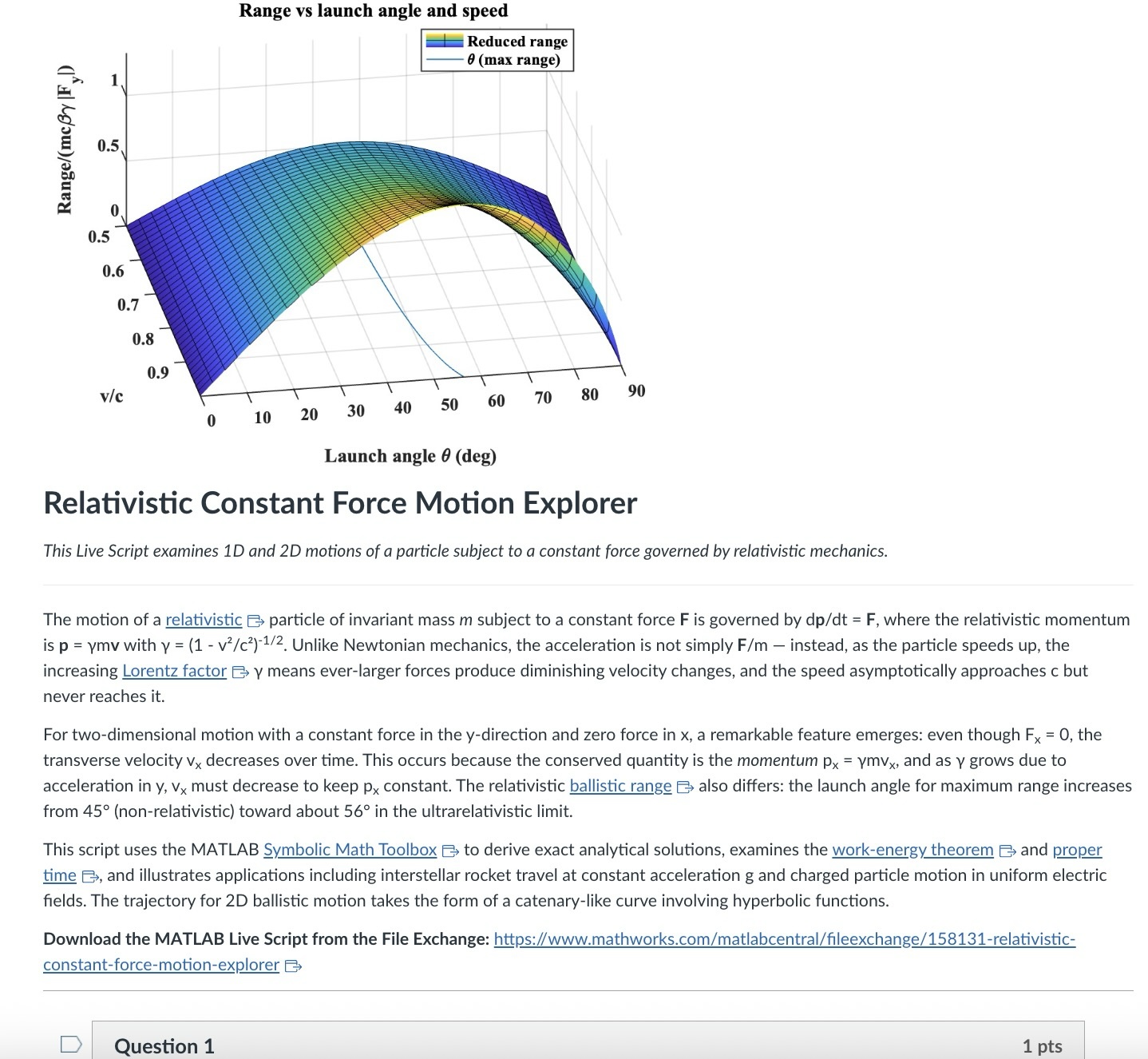
An AI-generated CANVAS quiz header based on a Live Script on relativistic motion.
Introduction
Agentic AI is disrupting higher education. An agentic AI can act on the web rather than relying solely on its training. It can research a topic and produce a credible research paper to specification with validated references. It can create, answer, or assess student work on physics questions from elementary mechanics to graduate-level quantum field theory or quantum computing. It can comprehend, generate, run, and debug a MATLAB Live Script zip package, an HTML5 interactive web application, a JavaScript-enabled website, an ADA-compliant CANVAS site with math and images, or a mobile phone app. A student can authenticate in a learning management system like CANVAS and issue a simple prompt to an agentic AI — “Complete all of my assignments in all of my courses. Thanks.” — and an instructor can, on the other side, with AI assistance and a simple prompt, assess all such submissions, even messy hand-written work. I have demonstrated these capabilities and others.
Here, I’d like to share an experiment leveraging AI to inject computation with MATLAB into a course in modern physics. This may interest the academic readers of this blog and the curious. My prior post Giving All Your Claudes the Keys to Everything introduced my personal agentic AI context.
Live Script goals
Some years back now, I started developing and introducing Live Scripts in a two-semester introductory physics course to immerse students in computation and science without sacrificing the rigor and breadth of the class. These students have essentially no background in computing and are exploring STEM majors — physics, astronomy, and engineering principally. A self-documenting Live Script allows a student to explore even a relatively advanced physics topic and data analysis trick like Fourier analysis or autocorrelation, using data like a mobile phone voice memo or a digital oscilloscope output race that they collect themselves, and then apply the same techniques to analyze big science open data from for example as gravitational wave observatory, both without being mired down in mathematics or code writing. As the course evolves, computational challenges connected to the laboratory component introduce much of the gamut of MATLAB functionality. The goal is to show why and how modeling and assessment using computation are essential in science, and to empower students with practical skills and a sense of what is possible. The traditional lecture/demonstration/homework/discussion format was largely untouched. This course sequence was a five-credit automatic honors course, so extra work was expected. Coding as a tool rather than a chore or vocation is all the more relevant in the AI age.
Assessment strategy
To flexibly direct and assess student work, each Live Script contains a variety of ‘Try this’ suggestions which require the user to adjust a parameter or two and observe the consequences. The student must study the physics described in the background information section, and the code enough to understand how the code logic works, using the supplied comments and URLs to documentation. Tackling a ‘Try this ‘ suggestion does not require any coding, just changing a parameter value, perhaps with a slider. Additionally, the Live Script contains ‘Challenges’ to extend the code in some simple or possibly advanced way. The Live Script can thus serve different customers, and an instructor can further tailor the script and embedded suggestions and challenges as they choose. The possibilities offered are only exemplary.
An associated CANVAS quiz contains a few multiple-choice questions related to the ‘Try this’ suggestions, which are auto-graded. Additional questions require the student to upload a product, like an appropriately labeled plot comparing data to a model fit, together with a written explanation. These are readily graded electronically using CANVAS SpeedGrader, with or without an e-rubric. The emphasis is on results and analysis, not on coding facility or style. By design, the burden on the instructor is minimal.
AI-generated computational thread
In teaching a 3-credit third-semester survey of modern physics (relativity, quantum mechanics, atomic, molecular, solid state, nuclear, particle, and astro physics) without a lab and again for students with little or no prior exposure to computation, I needed first to develop more advanced, relevant Live Scripts. This course offers three lecture hours per week, rife with live demonstrations of cathode ray tubes, electron diffraction, Geiger counters and sources, thermal radiation, the photoelectric effect, gas discharge tubes observed with diffraction glasses, lasers, and magnetic levitation with diamagnetic and high temperature superconductors, and so on. An additional mandatory hour per week is dedicated to small group active learning in sectional meetings. A contemporary e-text and integrated WebAssign homework system are linked via LTI to CANVAS. These components address learning goals I am loath to sacrifice. I ultimately decided to make the new computational thread an attractive extra-credit option (in parallel with a research paper option) and implemented it with AI assistance mid-stream this semester in a way that could be emulated.
The agent was Claude Desktop running with MCP servers: the Playwright browser-automation server (for CANVAS interaction via authenticated browser session), MATLAB MCP server to run MATLAB, and a filesystem server (for reading local Live Script packages and writing artifacts back to disk). I asked Claude to survey my modern physics syllabus on CANVAS and my 150+ Live Scripts on the MATLAB File Exchange (FEX), and to identify those relevant to a 3rd-semester course in relativity, quantum mechanics, atomic, molecular, solid state, nuclear, particle, and astro physics, with my Introduction to MATLAB script included as a foundations option. Claude returned an initial list of 38 candidate scripts. I removed two that were not a good fit and approved 14, including chaos in relativistic mechanics, relativistic motion in a Coulomb field, numerical solutions to the Schrödinger equation in 1D/2D/3D via the PDE Toolbox, gravitational-wave data analysis, exoplanet transit detection, and clustering in Gaia mission stellar data, among others.
For each approved script, Claude downloaded the FEX zip via MATLAB websave and unzip, converted the .mlx to readable .m text via matlab.internal.liveeditor.openAndConvert, ran the key numerical sections in MATLAB to obtain concrete answer values, and then used a single Playwright browser_evaluate call — authenticated by the CSRF token from the active CANVAS browser cookie — to POST a new quiz plus all of its questions to the CANVAS REST API in one round trip. (The MATLAB webwrite path with a CANVAS_API_TOKEN environment variable consistently returned 401 in our testing; the browser-session approach worked reliably for all 14 quizzes.)
Each quiz is structured identically: a description block with the FEX thumbnail image, a two- to three-paragraph physics introduction essentially copied from the FEX page or script itself with Wikipedia links to technical terms, a download link, and an “Open in MATLAB Online” link; followed by 4 multiple-choice questions worth 1 pt each (covering a fundamental physics fact, a physical mechanism, an experimental or computational technique, and a data-analysis concept), and 3 essay questions worth 3 pts each (a basic execution + screenshot, a quantitative comparison, and a bonus “Try this” modification). The essay type was deliberate: a CANVAS file_upload question accepts only a file, while an essay question gives the student a Rich Content Editor in which they can paste a screenshot directly from the clipboard and type their analysis in the same field. SpeedGrader then shows everything together. We also added an optional 0-credit student feedback question that we crafted jointly. Total: 13 points per quiz.
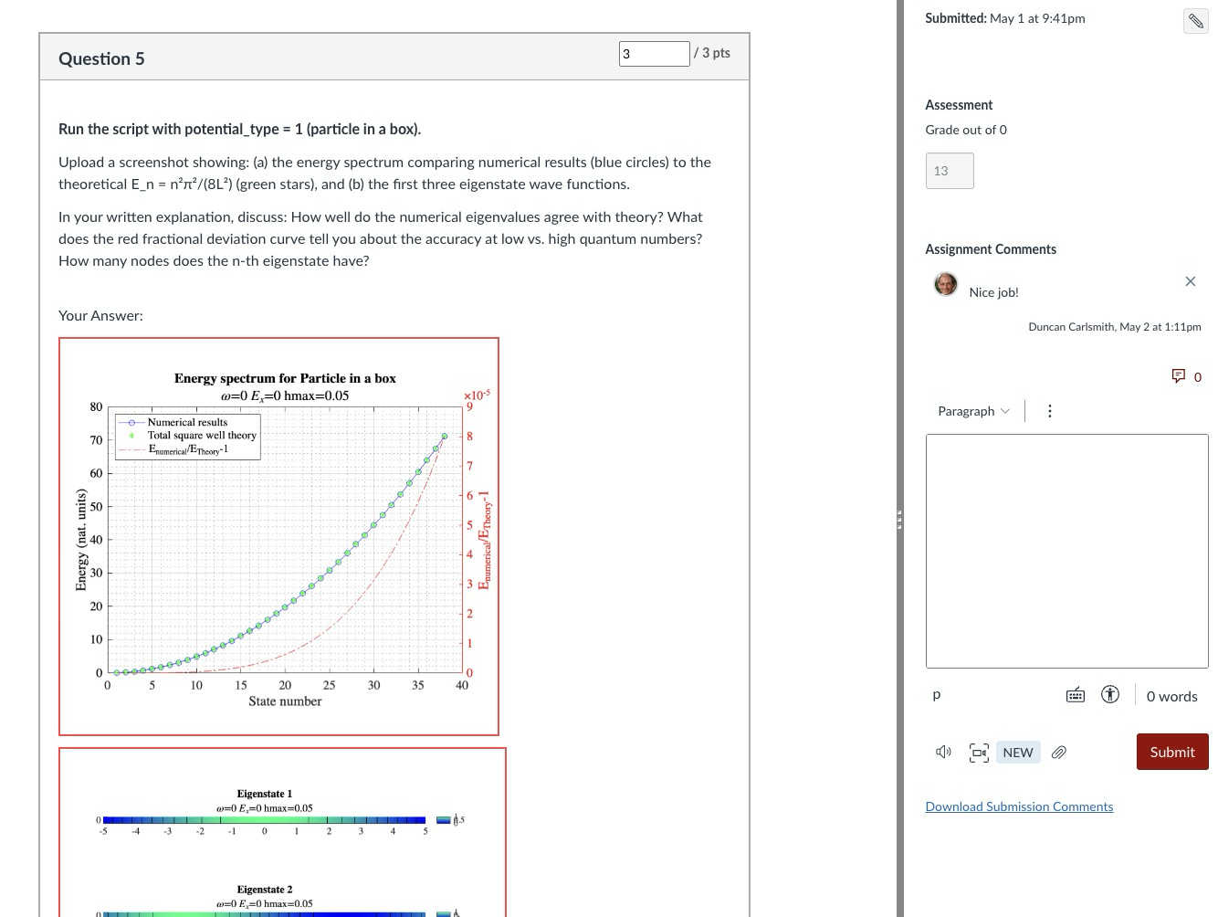
Speed Grader view of a Rich Content Editor question with uploaded results
The full set of 14 quizzes was created in a single working session. I reviewed and accepted the results essentially without revision — a few quiz descriptions needed a follow-up PUT to fix image sizing or to add the MATLAB Online link, but no question content required rewriting. Across the session, the procedure crystallized into a reusable SKILL.md that documents the FEX-to-CANVAS recipe end to end (download with MATLAB, design questions in the four-category MC pattern, batch quiz + question creation, verification checklist).
An AI touch on grading made the assignment fit the course without inflating its weight: a 5% group weight on the Computation category, with a drop-lowest-eleven-of-fourteen rule that keeps each student’s top three quizzes. Each quiz is 13 points, so the maximum contribution is (39/39) × 5% = 5.00% extra credit, and any student can attempt as few or as many as they wish without exceeding that cap. The CANVAS configuration is non-trivial in a few ways and includes one gotcha worth knowing about; details are in Appendix A.
Outcomes
I received about 75 submissions, with 30 of the 75 students participating, and many others opting for the research paper. Feedback was generally positive. Only a few students ran into difficulty: one suffered a European Space Agency network outage while accessing Gaia data, and another had trouble with a screen-capture process unrelated to MATLAB. Students reported workloads in an appropriate 1–3 hour range per assignment. Only about 20% of submitters elected to submit the (quite lengthy) Introduction to MATLAB assignment for credit; some likely encountered MATLAB already in the math department or engineering school, where it is used extensively, and others may have reviewed the assignment but elected not to submit because the upload questions concerned image processing (compression and decompression, blurring and deblurring) rather than course-relevant topics. Several students volunteered that these exercises were more informative and fun than their canonical problem-solving exercises.
Lessons
A few patterns from this experiment seem worth carrying forward. First, the ‘Try this’ design pattern that I had already adopted turns out to be unusually well suited to AI-assisted assessment: each suggestion converts almost mechanically into a three-part question (run, capture, analyze) with a defensible rubric; Hence one working session yielded a full term’s worth of quizzes. Second, the agentic build is a short, explicit recipe — read the script, run the calculations, design the questions, post via the CANVAS API in one batched call — that other instructors can replicate and which is now captured for me in a SKILL.md. Third, the Canvas grading mechanics (drop-lowest, keep-best-three, group weight cap) let extra-credit work scale gracefully: students self-select breadth versus depth, and the instructor’s exposure to grading volume is bounded.
Conclusions
More broadly, I expect education to become more efficient and engaging in this AI age, with much of the routine instructional and learning burden relegated to AI. Frontier AIs can affordably tutor undergraduate students and even PhDs at their level and challenge them in new ways and at scale. Students and instructors both must develop and adjust to new learning strategies and expectations. Documented exploration enabled by interactive, code-aware artifacts like Live Scripts and Jupyter notebooks, created by a student or researcher collaboratively with AIs and other compatriots, may play an ever more important role in this environment.
My SKILL.md is 665 lines and specific to my setup, so not shared here. You might be asking an AI to install Chromium and Playwright or Puppeteer and do all the work in its container. You might be electing a different assignment structure, accessing your own Live Scripts or Python equivalent located at GitHub or someplace other than the MATLAB FEX. This article documents most of what is in my skill file and would be useful background information. You will want to develop and test your own process if emulating the idea here.
Acknowledgements and disclosure
The products described here and this essay were prepared with the assistance of Claude.ai. The author declares he has no financial interest in Anthropic or MathWorks.
Appendix A: CANVAS gradebook configuration
The intent was simple to state: a student who completes three or more MATLAB quizzes at full marks should receive the full 5% extra-credit boost on their course total; a student who completes one quiz at full marks should receive one-third of that boost; a student who attempts none should receive nothing. Implementing this in CANVAS took three coordinated pieces, each of which is straightforward in isolation but has at least one non-obvious failure mode.
A.1 Group structure and drop rule. The 14 quizzes live in a single assignment group named “Computation,” weighted at 5% of the course grade. The group has one rule: drop the lowest 11 scores. With 14 assignments and 11 dropped, CANVAS keeps each student’s top three. Each quiz is worth 13 points (4 multiple-choice at 1 pt + 2 essay at 3 pts + 1 bonus essay at 3 pts), so the maximum sum across the kept three is 39, and the maximum group percentage is 39/39 = 100%, contributing 0.05 × 100% = 5.00% to the course total. The group weight thus acts as a hard ceiling: no matter how many quizzes a student attempts, their boost cannot exceed 5%.
A.2 Treating ungraded as zero, selectively. Out of the box, CANVAS treats ungraded assignments as ignored rather than as zero. This is usually the right default — a student who has not yet attempted an assignment is not penalized for it — but it interacts badly with the design intent here. If a student attempted exactly one MATLAB quiz and scored 13/13, CANVAS would show their Computation group total as 13/13 = 100%, awarding the full 5% boost for a single quiz. To get the intended scaling (one quiz at 13/13 should yield 13/39 = 33.33%, contributing 1.67% rather than 5%), the unattempted quizzes must count as zero in the group calculation.
The simplest way to enforce that globally is the gradebook setting Treat Ungraded as 0, but this applies course-wide and was undesirable in my case because of an exam-administration mixup in which different students had taken different versions of Exam 1; only the version each student took should count toward their exam grade, and a global “treat ungraded as 0” would have penalized students for the version they had not been assigned. The per-assignment alternative is to use the gradebook column menu (the three-dot menu on each assignment column) and choose Set Default Grade, entering 0 with the “Overwrite already-entered grades” box left unchecked. This converts every dash in that column to a 0 while leaving real scores untouched, and only affects the assignment whose menu was used. Applied to each of the 14 MATLAB quizzes, this gives the desired “ungraded as zero” behavior in the Computation group without affecting Exam 1 or any other category. After the fix, the worked examples behave as expected..
A.3 The points_possible gotcha. When a CANVAS Classic Quiz is created via the REST API and the quiz’s questions are POSTed in subsequent calls (or even, as in our case, in the same browser_evaluate call but as separate POST requests), the assignment row that mirrors the quiz in the gradebook can retain points_possible = 0 even though the questions internally sum to 13. The quiz preview displays the question points correctly, the quiz statistics show the correct totals, but the gradebook column header reads “Out of 0” and the group percentage calculation collapses to nonsense. Symptomatically, a student with one real score appeared at 30.77% in the Computation column when they should have been at 33.33% — the column was contributing 4/13 instead of 4/39 because 13 of the 14 columns were silently weightless.
The cure is to force CANVAS to recompute the assignment row’s points_possible from the question sum. The simplest way is per-quiz from the UI: open the quiz, click Edit, scroll to the bottom of the editor without changing anything, and click Save (not “Save & Publish” if the quiz is already published). The act of saving the quiz triggers the recompute. The same effect is available via the API by issuing PUT /api/v1/courses/{course_id}/assignments/{assignment_id} with body {"assignment": {"points_possible": 13}} on each affected assignment, which is faster for batch use.
The lesson for anyone scripting CANVAS quiz creation: after batch-creating quizzes and questions via the API, always verify the gradebook column header reads “Out of N” with N matching the question sum, and apply one of the two cures above before students start submitting. The skill file used in this project now flags this check explicitly.
Mitigating chat failures in AI code development
Duncan Carlsmith
Department of Physics, University of Wisconsin-Madison
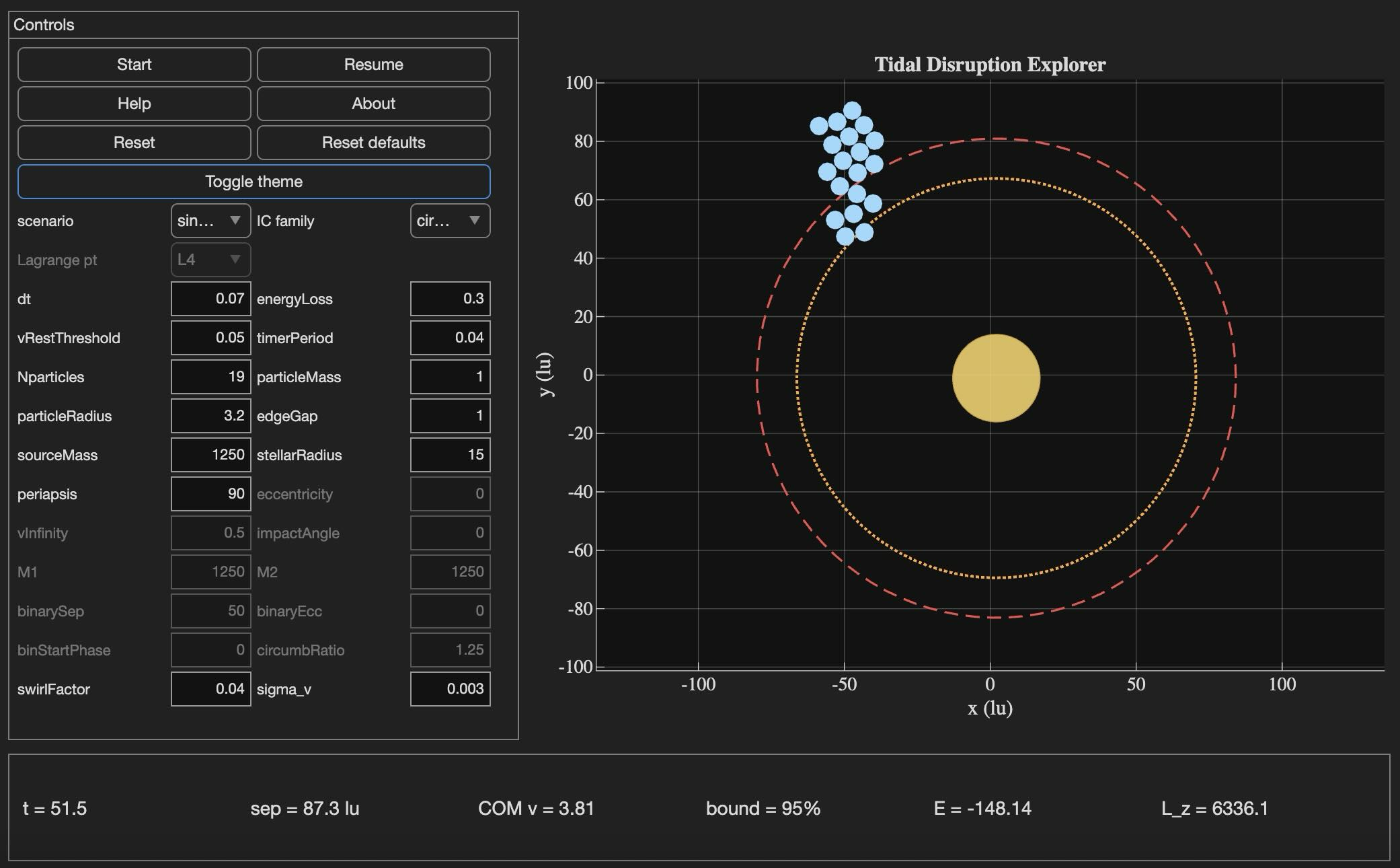
Tidal Disruption Explorer (MATLAB File Exchange 183760). The process of porting this Live Script ito HTML is described in this post.
Introduction
An agentic AI session ended for me this week with the message: "Claude is unable to respond to this request, which appears to violate our Usage Policy. Please start a new chat." Gulp. The substance of the conversation was completely benign — porting my MATLAB Live Script Tidal Disruption Explorer that simulates a self-gravitating cluster of particles being shredded by tidal forces near a massive object, like Comet Shoemaker-Levy 9 was shredded by Jupiter in 1992. The next chat picked up the work and finished it in seven turns.
Why nothing was lost is the subject of this post. The new product is the HTML5 port of Tidal Disruption Explorer and deployed at duncancarlsmith.github.io/TidalDisruptionExplorer-HTML5. But the more transferable product may be practices that can help make AI-assisted code development resilient to chat failures, connection drops, sandbox losses, and content-policy false positives. Two prior posts set my context: Live Script deployed as a 3D web application with AI introduced the workflow, and Giving All Your Claudes the Keys to Everything introduced the ngrok command server that makes the Mac controllable from any AI client. This post is about how to use such tools without losing your work when the chat dies.
Failure modes worth designing for
Long agentic sessions can fail in many ways, and most are out of the user's control. The bash_tool connection in the cloud container can go unresponsive mid-task. A stray Python process can mask a real command server on the same port. A lost development sandbox can vaporize generated artifacts — in an earlier turn of this same project, an entire test-harness directory disappeared with the sandbox and had to be reconstructed from the conversation log. Persistent context is not in fact persistent. Skills are forgotten. The user closes the laptop, the WiFi blinks off, or the chat hits a length limit. This project used Claude, but the problems are not AI-specific in my experience with 5-6 leading vendors. Without preparation, each of these is a real setback.
Best practices to consider
1. Externalize project state in a committed PROGRESS journal
A single file, committed in a repo, names every milestone, the test-pass count for each, the current state in prose, and an explicit "Recovery instructions for a fresh session" section that lists the source files, the test harness names, and the toolchain assumptions. When the previous chat failed, the next one resumed from this file alone, without needing the failed conversation. When the dev sandbox loss took out 10 test harnesses, they were rebuilt from the conversation log because the journal had recorded exactly what each harness checked and the expected pass count for each. These harnesses are also stored locally when complete and successful.
2. Two external locations:
The container contents are fragile even without a chat failure due to context compaction and hidden file management. I chose a local working directory as the editable source of truth. A GitHub repository was the final product and might have been used rather than my local storage - that choice was a matter of familiarity and trust. Each change was written locally first via the command server, verified on disk by reading it back, then committed and pushed to GitHub.
3. Run browser tests in the AI's container, not on the user's machine
For this project, the final product was a web app. In prior work, I used a local Chromium to view and test the product. It turns out that Claude's container ships with Node and Playwright preinstalled, and Chromium may be available from the Puppeteer install. Browser regression tests for the HTML5 application were run there entirely, and I only viewed staged intermediate products. Containing the development is not possible when building a MATLAB product without the added burden of using MATLAB in the cloud. The idea was to do as much as possible without overhead in the AI container.
4. Multistep plan with explicit approval gates
Decompose the work into milestones with sub-milestones. Each has a test harness with a documented expected pass count and a concrete deliverable. Don't merge "running a test" with "uploading the result" with "committing the change" — these separate decisions each has its own approval and verification. If the chat dies between any two of them or something else goes awry, the user can stop without leaving anything dangling. This project: 8 milestones, 27 sub-milestones, 260 documented sub-checks.
5. Versioned backups before any destructive write
Every PROGRESS edit got a timestamped pre-edit copy first in the local project repo, one per milestone.
Result
Recovery from the failed chat only cost me one turn. Six more turns to finish the project. The final result: 260 of 260 sub-checks pass across all milestones, live deployment verified. Many hairs pulled (the violation of usage policy issue was not the only one encountered!), but no utter despair experienced!
Links
Live HTML5 application: https://duncancarlsmith.github.io/TidalDisruptionExplorer-HTML5/
MATLAB Live Script (File Exchange 183760): https://www.mathworks.com/matlabcentral/fileexchange/183760-tidal-disruption-explorer
Source repository (GitHub): https://github.com/DuncanCarlsmith/TidalDisruptionExplorer-HTML5
Short version: MathWorks have released the MATLAB Agentic Toolkit which will significantly improve the life of anyone who is using MATLAB and Simulink with agentic AI systems such as Claude Code or OpenAI Codex. Go and get it from here: https://github.com/matlab/matlab-agentic-toolkit
Long version: On The MATLAB Blog Introducing the MATLAB Agentic Toolkit » The MATLAB Blog - MATLAB & Simulink
Have you ever wondered what it takes to send live audio from one computer to another? While we use apps like Discord and Zoom every day, the core technology behind real-time voice communication is a fascinating blend of audio processing and networking. Building a simple walkie-talkie is a perfect project for demystifying these concepts, and you can do it all within the powerful environment of MATLAB.
This article will guide you through creating a functional, real-time, push-to-talk walkie-talkie. We won't be building a replacement for a commercial radio, but we will create a powerful educational tool that demonstrates the fundamentals of digital signal processing and network communication.
The Purpose: Why Build This?
The goal isn't just to talk to a colleague across the office; it's to learn by doing. By building this project, you will:
Understand Audio I/O: Learn how MATLAB interacts with your computer’s microphone and speakers.
Grasp Network Communication: See how to send data packets over a local network using the UDP protocol.
Solve Real-Time Challenges: Confront and solve issues like latency, choppy audio, and continuous data streaming.
The Core Components
Our walkie-talkie will consist of two main scripts:
Sender.m: This script will run on the transmitting computer. It listens to the microphone when a key is pressed, sending the audio data in small chunks over the network.
Receiver.m: This script runs on the receiving computer. It continuously listens for incoming data packets and plays them through the speakers as they arrive.
Step 1: Getting Audio In and Out
Before we touch networking, let's make sure we can capture and play audio. MATLAB's built-in audiorecorder and audioplayer objects make this simple.
Problem Encountered: How do you even access the microphone?
Solution: The audiorecorder object gives us straightforward control.
code
% --- Test Audio Capture and Playback ---
Fs = 8000; % Sample rate in Hz
nBits = 16; % Number of bits per sample
nChannels = 1; % Mono audio
% Create a recorder object
recObj = audiorecorder(Fs, nBits, nChannels);
disp('Start speaking for 3 seconds.');
recordblocking(recObj, 3); % Record for 3 seconds
disp('End of Recording.');
% Get the audio data
audioData = getaudiodata(recObj);
% Play it back
playObj = audioplayer(audioData, Fs);
play(playObj);
Running this script confirms that your microphone and speakers are correctly configured and accessible by MATLAB.
Step 2: Sending Voice Over the Network
Now, we need to send the audioData to another computer. For real-time applications like this, the UDP (User Datagram Protocol) is the ideal choice. It’s a "fire-and-forget" protocol that prioritizes speed over perfect reliability. Losing a tiny packet of audio is better than waiting for it to be re-sent, which would cause noticeable delays (latency).
Problem Encountered: How do you send data continuously without overwhelming the network or the receiver?
Solution: We'll send the audio in small, manageable chunks inside a loop. We need to create a UDP Port object to handle the communication.
Here's the basic structure for the Sender.m script:
code
% --- Sender.m ---
% Define network parameters
remoteIP = '192.168.1.101'; % <--- CHANGE THIS to the receiver's IP
remotePort = 3000;
localPort = 3001;
% Create UDP Port object
udpSender = udpport("LocalPort", localPort, "EnablePortSharing", true);
% Configure audio recorder
Fs = 8000;
nBits = 16;
nChannels = 1;
recObj = audiorecorder(Fs, nBits, nChannels);
disp('Press any key to start transmitting. Press Ctrl+C to stop.');
pause; % Wait for user to press a key
% Start the Push-to-Talk loop
disp('Transmitting... (Hold Ctrl+C to exit)');
while true
recordblocking(recObj, 0.1); % Record a 0.1-second chunk
audioChunk = getaudiodata(recObj);
% Send the audio chunk over UDP
write(udpSender, audioChunk, "double", remoteIP, remotePort);
end
And here is the corresponding Receiver.m script:
code
Matlab
% --- Receiver.m ---
% Define network parameters
localPort = 3000;
% Create UDP Port object
udpReceiver = udpport("LocalPort", localPort, "EnablePortSharing", true, "Timeout", 30);
% Configure audio player
Fs = 8000;
playerObj = audioplayer(zeros(Fs*0.1, 1), Fs); % Pre-buffer
disp('Listening for incoming audio...');
% Start the listening loop
while true
% Wait for and receive data
[audioChunk, ~, ~] = read(udpReceiver, Fs*0.1, "double");
if ~isempty(audioChunk)
% Play the received audio chunk
play(playerObj, audioChunk);
else
disp('No data received. Still listening...');
end
end
Step 3: Solving Real-World Hurdles
Running the code above might work, but you'll quickly notice some issues.
Problem 1: Choppy Audio and High Latency
The audio might sound robotic or delayed. This is because of the buffer size and the processing time. Sending tiny chunks frequently can cause overhead, while sending large chunks causes delay.
Solution: The key is to find a balance.
Tune the Chunk Size: The 0.1 second chunk size in the sender (recordblocking(recObj, 0.1)) is a good starting point. Experiment with values between 0.05 and 0.2. Smaller values reduce latency but increase network traffic.
Use a Buffered Player: Instead of creating a new audioplayer for every chunk, we create one at the start and feed it new data. Our receiver code already does this, which is more efficient.
Problem 2: No Real "Push-to-Talk"
Our sender script starts transmitting and doesn't stop. A real walkie-talkie only transmits when a button is held down.
Solution: Simulating this in a script requires a more advanced technique, ideally using a MATLAB App Designer GUI. However, we can create a simple command-window version using a figure's KeyPressFcn.
Here is an improved concept for the Sender that simulates radio push-to-talk, e.g. https://www.retevis.com/blog/ptt-push-to-talk-walkie-talkies-guide
% --- Advanced_Sender.m ---
function PushToTalkSender()
% -- Configuration --
remoteIP = '192.168.1.101'; % <--- CHANGE THIS
remotePort = 3000;
localPort = 3001;
Fs = 8000;
% -- Setup --
udpSender = udpport("LocalPort", localPort);
recObj = audiorecorder(Fs, 16, 1);
% -- GUI for key press detection --
fig = uifigure('Name', 'Push-to-Talk (Hold ''t'')', 'Position', [100 100 300 100]);
fig.KeyPressFcn = @KeyPress;
fig.KeyReleaseFcn = @KeyRelease;
isTransmitting = false; % Flag to control transmission
disp('Focus on the figure window. Hold the ''t'' key to transmit.');
% --- Main Loop ---
while ishandle(fig)
if isTransmitting
% Non-blocking record and send would be ideal,
% but for simplicity we use short blocking chunks.
recordblocking(recObj, 0.1);
audioChunk = getaudiodata(recObj);
write(udpSender, audioChunk, "double", remoteIP, remotePort);
disp('Transmitting...');
else
pause(0.1); % Don't burn CPU when idle
end
drawnow; % Update figure window
end
% --- Callback Functions ---
function KeyPress(~, event)
if strcmp(event.Key, 't')
isTransmitting = true;
end
end
function KeyRelease(~, event)
if strcmp(event.Key, 't')
isTransmitting = false;
disp('Transmission stopped.');
end
end
end
Conclusion and Next Steps
You've now built the foundation of a real-time voice communication tool in MATLAB! You've learned how to capture audio, send it over a network using UDP, and handle some of the fundamental challenges of real-time streaming.
This project is the perfect starting point for more advanced explorations:
Build a Full GUI: Use App Designer to create a user-friendly interface with a proper push-to-talk radio button.
Implement Noise Reduction: Apply a filter (e.g., a simple low-pass or a more advanced spectral subtraction algorithm) to the audioChunk before sending it.
Add Channels: Modify the code to use different UDP ports, allowing users to select a "channel" to talk on.
In a previous discussion,
we looked at a variety of infallible tests for primality, but all of them were too slow to be viable for large numbers. In fact, all of the methods discussed there will fail miserably for even moderately large numbers, those with just a few dozen decimal digits. That does not even begin to push into the realm of large numbers. In turn, that forces us into a different realm of tests - tests which are usually and even almost always correct, but can sometimes incorrectly predict primality.
In this discussion, I will be trying to convince you that the Fermat test for primality can be a quite good test when the number is sufficiently large. Except of course, when it is really bad. Even so, the Fermat test for primality is both a useful tool as well as a necessary underpinning for several other better tests.
The Fermat test for primality relies on Fermat's little theorem, a perhaps under-appreciated tool. Even the name implies it is of little interest. I'm not taking about the famous last theorem, only proven in recent years, but his little theorem.
If you want to look over some nice ways to prove the little theorem, take a read in this link:
I will readily admit that long ago, when I learned about the little theorem in a nearly forgotten class, I thought it was interesting, but why would I care? Not until I learned more mathematics and saw Fermat’s little theorem appearing in different places did I begin to appreciate it. Fermat tells us that, IF P is a prime, AND w is co-prime with P (so the two are relatively prime, sharing no common factors except 1), then it must be true that
mod(w^(P-1),P) == 1
Try it out. Does it work? Be careful though as too large of an exponent will cause problems in double precision, and that is not difficult to do. As a test case that will not overwhelm doubles, note that 13 is prime, and 3 shares no common factors with 13, so we satisfy the requirements for Fermat's little theorem.
mod(3^12,13)
We can even verify that any co-prime of 13 will yield the same result.
mod((1:12).^12,13)
Indeed it worked, suggesting what we knew all along, that 13 is prime. The little Fermat test for primality of the number P uses a converse form of Fermat's little theorem, thus given a co-prime number w known as the witness, is that if
mod(w^(P-1),P)==1
then we have evidence that P is indeed prime. This is not conclusive evidence, but still it is evidence. It is not conclusive because the converse of a true statement is not always true.
The analogy I like here is if we lived in a universe where all crows are black. (I'll ask you to pretend this is true. In fact, some crows have a mutation, making them essentially albino crows. For the purposes of this thought experiment, pretend this cannot happen.) Now, suppose I show you a picture of a bird which happens to be black. Do you know the bird to be a crow? Of course not, as the bird may be a raven, or a redwing blackbird (until you see the splash of red on the wing), a common grackle, a European starling in summer plumage, a condor, etc. But having seen black plumage, it is now more likely the bird is indeed a crow. I would call this a moderately weak evidentiary test for crow-ness.
Little Fermat may seem to be of little value when testing for primality for two reasons. First, computing the remainder would seem to be highly CPU intensive for large P. In the example above, I had only to compute 3^12=531441, which is not that large. But for numbers with many thousands or millions of digits, directly raising even a number as small as 2 to that power will overwhelm any computer. Secondly, if we do that computation, little Fermat does not conclusively prove P to be prime.
Our savior in one respect is the powermod tool. And that helps greatly, since we can compute the remainder in a reasonable time. A powermod call is quite fast even for huge powers. (I won't get into how powermod works here, since that alone is probably worth a discussion. I could though, if I see some interest because there are some very pretty variations of the powermod algorithm. I hope to show you one of them when I discuss the Fibonacci test for primality in a future post.) Trying the little Fermat test using powermod on a number with 1207 decimal digits, I’ll first do a time check.
P = 4000*sym(2)^3999 - 1;
timeit(@() powermod(2,P-1,P))
As you can see, powermod really is pretty fast. Compared to an isprime test on that number it would show a significant difference.
I have said before that little Fermat is not a conclusive test. In fact, a good trick is to perform a second little Fermat test, using a different witness. If the second test also indicates primality, then we have additional evidence that P is in fact prime.
w = [2 3]; % Two parallel witnesses
powermod(w,P-1,P)
This value for P is indeed prime, and little Fermat suggests it is, doubly suggestive in that test since I actually performed two parallel tests. Here however, we need to understand when it will fail, and how often it will fail.
If we perform a little Fermat test for primality, we will never see false negatives, that is, if any test with any witness ever indicates a number is composite, then it is certainly composite. (The contrapositive of a true statement is always true.) The alternate class of failure is the false positive, where little Fermat indicates a number is prime when it was actually composite.
If P is composite, and w co-prime with P, we call P a Fermat pseudo-prime for the witness w if we see a remainder of 1 when P was in fact composite. When that happens, the witness (w) is called a Fermat liar for the primality of P. (A list of some Fermat pseudo-primes where 2 is a Fermat liar can be found in sequence A001567 of the OEIS.)
In the case of 4000*2^3999-1, I claimed the number to be in fact prime, and it was identified so (as PROBABLY prime by little Fermat. Next, consider another number from that same family. I’ll perform three parallel tests on it, with witnesses 2, 3, and 5. This will suggest the value of doing parallel tests on a number to reduce the failure rate from little Fermat.
P2 = 1024*sym(2)^1023 - 1;
w = [2; 3; 5];
gcd(w,P2)
F2 = powermod(w,P2-1,P2)
logical(F2 == 1)
As you can see, P2 is co-prime with all of 2, 3 and 5, but 2 is a Fermat liar, whilst 3 and 5 are Fermat truth tellers, identifying P2 as certainly composite. So the little Fermat test can definitely fail for SOME witnesses, since we see a disagreement. However, an interesting fact about P2 above is it is also a Mersenne number with prime exponent, thus it can be written as 2^1033-1, where 1033 is prime. I can go into more detail about this case later, but we can show that 2 is always a Fermat liar for composite Mersenne numbers when the exponent is itself prime. I’ll try to leave more detail on this matter in a future discussion, or perhaps a comment.
Next, consider the composite integer 51=3*17. As the product of two primes, it is clearly not itself prime.
P51 = 51;
w0 = 2:P51-2;
w = w0(gcd(w0,P51) == 1)
Note that I did not include 1 or 50 in that set, since 1 raised to any power is 1, and 50 is congruent to -1, mod 51. -1 raised to any even power is also always 1, and 51-1 is an even number. And so when we are working modulo 51, both 1 and 50 are not useful witnesses in terms of the little Fermat test.
R = powermod(w,P-1,P)
w(R == 1)
This teaches us that when 51 is tested for primality using the little Fermat test, there are 2 distinct witnesses w (16 and 35) we could have chosen which would have been Fermat liars, but all 28 other potential co-prime witnesses would have been truth tellers, accurately showing 51 to be composite. Proportionally, little Fermat will have been correct roughly 93% of the time, since only 2 of these 30 possible tests returned a false positive. (I’ll add that for any modulus P, if w<P is not co-prime with the modulus, then the computation mod(w^(P-1),P) will always return a non-unit result, and therefore we can theoretically use any integer w from the set 2:P-2 as a witness. However if w is co-prime with P then P is clearly not prime, and the entire problem becomes a little less interesting. As such, I will only consider co-prime witnesses for this discussion.) Regardless, that would make the little Fermat test for P=51 even more often correct, since it returns the correct result of composite for 46 out of the 48 possible witnesses 2:49. Does this mean Little Fermat is indeed the basis for a good test to rely on to learn if a number is prime? Well, yes. And no.
Little Fermat forms a very good test most of the time, but reliance is a strong word. This means we need to explore the little Fermat test in more depth, focusing on Fermat liars and the case of false positives. To offer some appreciation of the false positive rate, offline, I have tested all composite integers between 4 and 10000, for all their possible co-prime witnesses.
load FermatLiarsData
In that .mat file, I've saved three vectors, X, witnessCount, and liarCount. X is there just to use for plotting purposes and is NaN for all non-composite entries.
whos X witnessCount liarCount
The vector witnessCount is the number of valid witnesses for the corresponding number in X. Corresponding to that is the vector liarCount, which is the number of Fermat liars I found for each composite in X.
How many Fermat test useful witnesses are there for any integer X? This is just 2 less than the number of coprimes of X. The number of coprimes is given by the Euler totient function, commonly called phi(X). (I’ll be going into more depth on the totient in the next chapter of this series, because the Euler totient is a crucial part of understanding how all of this works.)
The witness count is phi(X)-2. Why subtract 2? 1 can never be a witness, but 1 is technically coprime to everything. The same applies to X-1 (which is congruent to -1 mod X.) As such, there are phi(X)-2 coprimes to consider. (I've posted a function called totient on the FEX, but it is easily computed if you know the factorization of X. Or for small numbers, you can just use GCD to identify all co-primes, and count them.)
plot(X,witnessCount,'.')
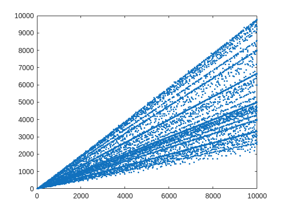
From that plot, you can learn a few interesting things. (As a mathematician, this is what I love the most, thus to look at whay may be the simplest, most boring plot, and try to find something of value, something I had never thought of before.) For example, we know that when X is prime, then everything from the set 2:X-2 is a valid witness. So the upper boundary on that plot will be the line y==x. As well, there are a few numbers where the order of the set of witnesses will be close to the maximum possible. For example, 961=31*31, has 928 valid witnesses. That makes some sense, as 961 is the square of a prime (31), so we know 961 is divisible only by 31. Only multiples of 31 will not be coprime with 961.
But how about the lower boundary? The least number of valid witnesses will always come from highly composite numbers, because they will share common factors with almost everything. For example 30 = 2*3*5, or 210=2*3*5*7.
witnessCount([30 210 420])
A good discussion about the lower bound for that plot can be found here:
What really matters to us though, is the fraction of the useful witnesses for a little Fermat test that yield a false positive.
plot(X,liarCount./witnessCount,'b.')
Cind = liarCount == witnessCount;
hold on
plot(X(Cind),1,'ro')
ylabel('Liar fraction')
xlabel('X')
title('Fermat pseudo-prime strength')
hold off
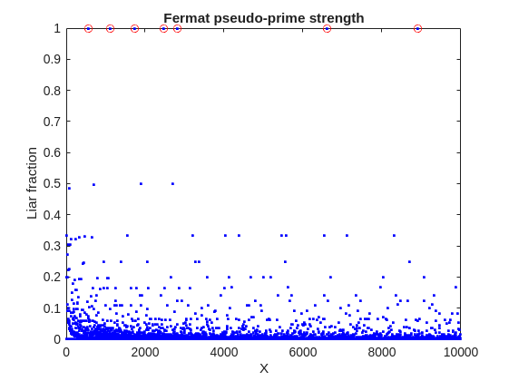
A look at this plot shows seven circles in red, corresponding to X from the list {561, 1105, 1729, 2465, 2821, 6601, 8911} which are collectively known as Carmichael numbers. These are numbers where all witnesses return a false positive. Carmichael numbers are themselves fairly rare. You can find a list of them as sequence A002997 in the OEIS. And for those of you who have never wandered around the OEIS, please take this opportunity to do so now. The OEIS stands for Online Encyclopedia of Integer Sequences. It contains a wealth of interesting knowledge about integers and integer sequences.)
There are a few other interesting numbers we can find in that plot, like 91 and 703, where roughly 50% of the valid witnesses yield false positives. Of the complete set, which numbers did return at least a 25% false positive rate for primality? These numbers would be known as strong pseudo-primes for the little Fermat test, because they are pseudo-primes for at least 25% of the potential witnesses. These strong pseudo-primes have some interesting similarities to the Carmichael numbers. (My next post will go into more depth on Carmichael numbers and strong pseudo-primes. At the moment, I am merely interested in looking at the how often the little Fermat test fails overall.)
find(liarCount./witnessCount> 0.25)
You should notice the spacing between successive strong Fermat pseudo-primes is growing slowly, with a spacing of roughly 800 on average in the vicinity of 10000. If I step out beyond by a factor of 10, the next strong Fermat pseudo-primes after 1e5 are {101101, 104653, 107185, 109061, 111361, 114589, 115921 126217, 126673}, so that average spacing is definitely growing.
Given that set, now we can look at the prime factorizations of each of those strong pseudo-primes. Can we learn something about them?
arrayfun(@factor,find(liarCount./witnessCount> 0.25),'UniformOutput',false)
Perhaps the most glaring thing I see in that set of factors is almost all of those strong Fermat pseudo-primes are square free. That is, in that list, only 45=3*3*5 had any replicated factor at all. That property of being square free is something we will see is necessary to be a Carmichael number, but it also suggests that a simple roughness test applied in advance would have eliminated almost all of those strong pseudo-primes as obviously not prime, even at a very low level of roughness.
In fact, for most composite integers, most witnesses do indeed return a negative, indicating the number is not prime, and therefore composite. Little Fermat does not commonly tell falsehoods, even though it can do so.
semilogy(X,movmedian(liarCount./witnessCount,20,'omitnan'),'b-')
title('False positive fraction for composites')
yline(0.0003,'r')

We can learn from this last plot that as the number to be tested grows large, the median false positive rate for little Fermat, even for X as low as only 10000, is roughly 0.0003. (It continues to decrease for larger X too. In fact, I’ve read that when X is on the order of 2^256, the relative fraction of Fermat liars is on the order of 1 in 1e12, and it continues to decrease as X grows in magnitude. In my eyes, that seems pretty good for an imperfect test. Not perfect, but not bad when paired with roughness and perhaps a second little Fermat test using a different witness, and we will start to see tests which bear a higher degree of strength.)
I’ll stop at this point in this post because the post is getting lengthy. In my next post, I’d like to visit some questions about what are Carmichael numbers, about whether some witnesses are better than others, and if there are any numbers which lack any Fermat liars. However, in order to dive more deeply, I will need to explain how/why/when the little Fermat test works, and what causes Fermat liars. Stay tuned, because this starts to get interesting.
Hi everyone,
Some of you may remember my earlier post. Quick version: I'm a biomed PhD student, I use MATLAB daily, and I noticed that AI coding tools often suggest functions that don't exist in R2025b or use deprecated ones. So I built skills that teach them what actually works.
v2.0 adds 54 template `.m` scripts, rewrites all knowledge cards based on blind testing, and verifies every function call against live MATLAB. I tested each skill on 17 prompts and caught 8 hallucinated functions across 5 toolboxes (Medical Imaging, Deep Learning, Image Processing, Stats-ML, Wavelet).
Give it a spin!
Repo: matlab-toolbox-skills
The skills follow the Agent Skills open standard, so they also work with Codex, Gemini CLI, Claude Code and others. If you use the official Matlab MCP Server from MathWorks, these skills complement it: the MCP server executes your code, the skills help the AI write good code to begin with.
One ask
How do we measure performance and evaluate agent skills? We can run blind tests and catch hallucinated functions, but that only covers what we thought to test. The honest answer is that the best way to evaluate these is community consensus and real-world testimonials. How are you using them? What worked? What still broke?
Your use cases and feedback are the most reliable eval I can get, and as a student building this, they're also the real motivation for me to keep going. If a skill saved you from a hallucinated function or pointed you to the right function call, I'd love to hear about it. If something is still wrong, I need to hear about it.
Issues, PRs, or just a reply here. Star the repo if it saved you time.
Thanks!
Happy Spring! and Happy Coding in Matlab!
Best,
Ritish
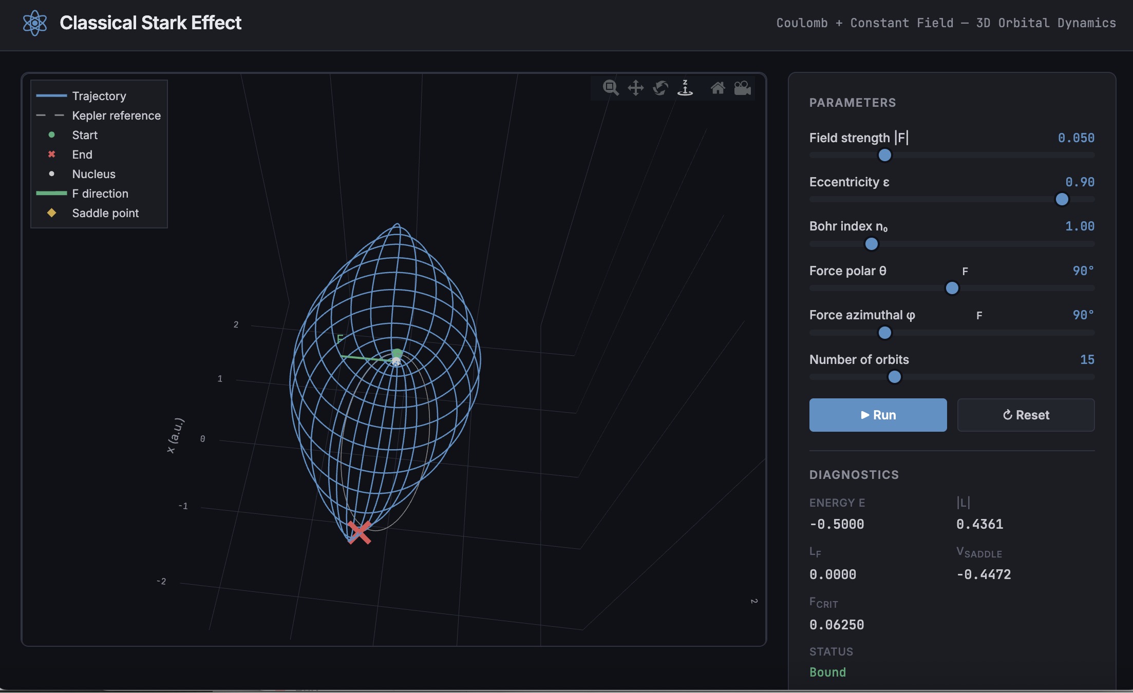
A Live Script can be converted to an HTML5 framework web application with AI as described in Double Pendulum Chaos Explorer: From HTML5 Prototype to MATLAB interactive application with AI. I have recently provides converted the Live Script Classical Stark Effect to a web application supporting a 3D twirlable display of motion of a particle subject to an inverse square law force plus an additional constant force - the problem known as the classical Stark effect.
The web application deployed to GitHub may be launched here and documents its dependencies below the interactive application. The files are available at Classical Stark Effect — Interactive Web Simulation. One gotcha was the need to enable hardware acceleration in Chrome (no problem in Safari) to support a 3D twirlable display. If hardware acceleration is disabled in Chrome, the application provides a warning and replaces the 3D twirlable display with a 2D alternate.
The conversion of the script to a web application was performed with Perplexity.ai. The GitHub deployment was accomplished with Anthropic's Claude using the open source GitHub CLI. WIth the gh CLI (already installed and authenticated on my Mac) via osascript, and Claude connected to my file system via MCP and an ngrok server, Claude executed on my Mac the following sequence of steps:
1. git init
Creates a hidden .git/ directory in the staging folder, initializing it as a local git repository. Before this command the folder is just a plain directory; after it, git can track files there. Run once per new project.
2. git branch -M main
Renames the default branch to main. Older git versions default to master; GitHub now expects main. The -M flag forces the rename even if main already exists. Must run after git init and before the first commit.
3. git add -A
Stages all files in the directory tree for the next commit. The -A flag means "all" -- new files, modified files, and deleted files are all included. This does not write anything to GitHub; it only updates git's internal index (the staging area) on your local machine.
4. git commit -m 'Initial release: Classical Stark Effect Interactive Simulation'
Takes everything in the staging area and freezes it into a permanent commit object stored in .git/. This is the snapshot that will be pushed. The -m flag provides the commit message inline. After this command, git knows exactly what files exist and what their contents are -- gh repo create --push will send exactly this snapshot.
5. gh repo create ClassicalStarkEffect --public --source=. --push
Three things happen in sequence inside this one command:
- gh repo create ClassicalStarkEffect --public -- calls the GitHub API to create a new empty public repository named ClassicalStarkEffect under the authenticated account (DuncanCarlsmith).
- --source=. -- tells gh to treat the current directory as the local git repo. It reads .git/ to find the commits and configures the remote.
- --push -- sets the new GitHub repo as origin and runs the equivalent of git push origin main, sending the commit from step 4 up to GitHub.
Without steps 1-4 having run first, --push would have nothing to send and the repo would land empty.
6. gh api repos/DuncanCarlsmith/ClassicalStarkEffect/pages --method POST -f build_type=legacy -f source[branch]=main -f 'source[path]=/'
Calls the GitHub REST API directly to enable GitHub Pages on the repo. Breaking down the flags:
- --method POST -- this is a create operation (not a read), so it uses HTTP POST.
- -f build_type=legacy -- critical flag. Tells GitHub to serve files directly from the branch. The alternative (workflow) would expect a .github/workflows/ Actions file to build and deploy the site, which doesn't exist here, and would produce a permanent 404.
- -f source[branch]=main -- serve from the main branch.
- -f 'source[path]=/' -- serve from the root of the branch (as opposed to a /docs subdirectory).
This is the API equivalent of going to Settings > Pages in the GitHub web UI and setting Branch: main, Folder: / (root), clicking Save.
7. curl -s -o /dev/null -w "%{http_code}" https://duncancarlsmith.github.io/ClassicalStarkEffect/
Not a git or gh command, but the verification step. GitHub Pages takes ~60 seconds to build after step 6. This curl fetches the live URL and prints only the HTTP status code (-w "%{http_code}"), discarding the body (-o /dev/null) and suppressing progress output (-s). 200 means live; 404 means still building.