Results for
Hey cody fellows :-) !
I recently created two problem groups, but as you can see I struggle to set their cover images :
What is weird given :
- I already did it successfully twice in the past for my previous groups ;
- If you take one problem specifically, Problem 60984. Mesh the icosahedron for instance, you can normally see the icon of the cover image in the top right hand corner, can't you ?
- I always manage to set cover images to my contributions (mostly in the filexchange).
I already tried several image formats, included .png 4/3 ratio, but still the cover images don't set.
Could you please help me to correctly set my cover images ?
Thank you.
Nicolas
Is there a hardware support package available for the MP series?
t = turtle(); % Start a turtle
t.forward(100); % Move forward by 100
t.backward(100); % Move backward by 100
t.left(90); % Turn left by 90 degrees
t.right(90); % Tur right by 90 degrees
t.goto(100, 100); % Move to (100, 100)
t.turnto(90); % Turn to 90 degrees, i.e. north
t.speed(1000); % Set turtle speed as 1000 (default: 500)
t.pen_up(); % Pen up. Turtle leaves no trace.
t.pen_down(); % Pen down. Turtle leaves a trace again.
t.color('b'); % Change line color to 'b'
t.begin_fill(FaceColor, EdgeColor, FaceAlpha); % Start filling
t.end_fill(); % End filling
t.change_icon('person.png'); % Change the icon to 'person.png'
t.clear(); % Clear the Axes
classdef turtle < handle
properties (GetAccess = public, SetAccess = private)
x = 0
y = 0
q = 0
end
properties (SetAccess = public)
speed (1, 1) double = 500
end
properties (GetAccess = private)
speed_reg = 100
n_steps = 20
ax
l
ht
im
is_pen_up = false
is_filling = false
fill_color
fill_alpha
end
methods
function obj = turtle()
figure(Name='MATurtle', NumberTitle='off')
obj.ax = axes(box="on");
hold on,
obj.ht = hgtransform();
icon = flipud(imread('turtle.png'));
obj.im = imagesc(obj.ht, icon, ...
XData=[-30, 30], YData=[-30, 30], ...
AlphaData=(255 - double(rgb2gray(icon)))/255);
obj.l = plot(obj.x, obj.y, 'k');
obj.ax.XLim = [-500, 500];
obj.ax.YLim = [-500, 500];
obj.ax.DataAspectRatio = [1, 1, 1];
obj.ax.Toolbar.Visible = 'off';
disableDefaultInteractivity(obj.ax);
end
function home(obj)
obj.x = 0;
obj.y = 0;
obj.ht.Matrix = eye(4);
end
function forward(obj, dist)
obj.step(dist);
end
function backward(obj, dist)
obj.step(-dist)
end
function step(obj, delta)
if numel(delta) == 1
delta = delta*[cosd(obj.q), sind(obj.q)];
end
if obj.is_filling
obj.fill(delta);
else
obj.move(delta);
end
end
function goto(obj, x, y)
dx = x - obj.x;
dy = y - obj.y;
obj.turnto(rad2deg(atan2(dy, dx)));
obj.step([dx, dy]);
end
function left(obj, q)
obj.turn(q);
end
function right(obj, q)
obj.turn(-q);
end
function turnto(obj, q)
obj.turn(obj.wrap_angle(q - obj.q, -180));
end
function pen_up(obj)
if obj.is_filling
warning('not available while filling')
return
end
obj.is_pen_up = true;
end
function pen_down(obj, go)
if obj.is_pen_up
if nargin == 1
obj.l(end+1) = plot(obj.x, obj.y, Color=obj.l(end).Color);
else
obj.l(end+1) = go;
end
uistack(obj.ht, 'top')
end
obj.is_pen_up = false;
end
function color(obj, line_color)
if obj.is_filling
warning('not available while filling')
return
end
obj.pen_up();
obj.pen_down(plot(obj.x, obj.y, Color=line_color));
end
function begin_fill(obj, FaceColor, EdgeColor, FaceAlpha)
arguments
obj
FaceColor = [.6, .9, .6];
EdgeColor = [0 0.4470 0.7410];
FaceAlpha = 1;
end
if obj.is_filling
warning('already filling')
return
end
obj.fill_color = FaceColor;
obj.fill_alpha = FaceAlpha;
obj.pen_up();
obj.pen_down(patch(obj.x, obj.y, [1, 1, 1], ...
EdgeColor=EdgeColor, FaceAlpha=0));
obj.is_filling = true;
end
function end_fill(obj)
if ~obj.is_filling
warning('not filling now')
return
end
obj.l(end).FaceColor = obj.fill_color;
obj.l(end).FaceAlpha = obj.fill_alpha;
obj.is_filling = false;
end
function change_icon(obj, filename)
icon = flipud(imread(filename));
obj.im.CData = icon;
obj.im.AlphaData = (255 - double(rgb2gray(icon)))/255;
end
function clear(obj)
obj.x = 0;
obj.y = 0;
delete(obj.ax.Children(2:end));
obj.l = plot(0, 0, 'k');
obj.ht.Matrix = eye(4);
end
end
methods (Access = private)
function animated_step(obj, delta, q, initFcn, updateFcn)
arguments
obj
delta
q
initFcn = @() []
updateFcn = @(~, ~) []
end
dx = delta(1)/obj.n_steps;
dy = delta(2)/obj.n_steps;
dq = q/obj.n_steps;
pause_duration = norm(delta)/obj.speed/obj.speed_reg;
initFcn();
for i = 1:obj.n_steps
updateFcn(dx, dy);
obj.ht.Matrix = makehgtform(...
translate=[obj.x + dx*i, obj.y + dy*i, 0], ...
zrotate=deg2rad(obj.q + dq*i));
pause(pause_duration)
drawnow limitrate
end
obj.x = obj.x + delta(1);
obj.y = obj.y + delta(2);
end
function obj = turn(obj, q)
obj.animated_step([0, 0], q);
obj.q = obj.wrap_angle(obj.q + q, 0);
end
function move(obj, delta)
initFcn = @() [];
updateFcn = @(dx, dy) [];
if ~obj.is_pen_up
initFcn = @() initializeLine();
updateFcn = @(dx, dy) obj.update_end_point(obj.l(end), dx, dy);
end
function initializeLine()
obj.l(end).XData(end+1) = obj.l(end).XData(end);
obj.l(end).YData(end+1) = obj.l(end).YData(end);
end
obj.animated_step(delta, 0, initFcn, updateFcn);
end
function obj = fill(obj, delta)
initFcn = @() initializePatch();
updateFcn = @(dx, dy) obj.update_end_point(obj.l(end), dx, dy);
function initializePatch()
obj.l(end).Vertices(end+1, :) = obj.l(end).Vertices(end, :);
obj.l(end).Faces = 1:size(obj.l(end).Vertices, 1);
end
obj.animated_step(delta, 0, initFcn, updateFcn);
end
end
methods (Static, Access = private)
function update_end_point(l, dx, dy)
l.XData(end) = l.XData(end) + dx;
l.YData(end) = l.YData(end) + dy;
end
function q = wrap_angle(q, min_angle)
q = mod(q - min_angle, 360) + min_angle;
end
end
end
Nice to have - function output argument provide code assist when said function is called
This is a feature which doesn't apear to currently exist, but I think alot of matlab users would like, particularly ones who write alot of custom classes.
Imagine i have a custom class with some properties:
classdef CustomClass < handle
properties
name (1,1) string = "default name"
varOne (1,1) double = 0
end
methods
function obj = CustomClass(name,varOne)
obj.name = name;
obj.VarOne = varOne;
end
end
end
Then imagine I have a function which returns one of these custom class objects:
function [obj] = Calculation(Var1,Var2,name)
arguments (Input)
Var1 (1,1) double
Var2 (1,1) double
end
arguments (Output)
obj (1,1) CustomClass
end
results = Var1 + Var2;
obj = CustomClass(name,result);
end
With this class and this function which returns one of these class objects, I would like the fact that I provided "(1,1) CustomClass" in the output arguemnts block of function "Calculation(Var1,Var2,name)" to trigger code assist automaticaly show me, when writing code that the retuned value from this funciton has properties "name" and "varOne" in the object.
For istance, if I write the following code with this function and the class in the Matlab search path
testObj = Calculation(1,1,"test");
testObj.varOne = 10; %the property "varOne" doesn't apear in code assist when writing this line of code
I would like that the fact function "Calcuation(Var1,Var2,name) has the output arguments block enforcing that this function must return an object of "CustomClass" to make code assist recognise that "testObj" is a "CustomClass" object, just as if testObj was an input argument to another function which had an input argument requiring that "testObj" was a "CustomClass" object.
Maybe this is a feature that may be added to matlab in future releases? (please and thank you LOL)
I would like to zoom directly on the selected region when using  on my image created with image or imagesc. First of all, I would recommend using image or imagesc and not imshow for this case, see comparison here: Differences between imshow() and image()? However when zooming Stretch-to-Fill behavior happens and I don't want that. Try range zoom to image generated by this code:
fig = uifigure;
ax = uiaxes(fig);
im = imread("peppers.png");
h = imagesc(im,"Parent",ax);
axis(ax,'tight', 'off')
I can fix that with manualy setting data aspect ratio:
daspect(ax,[1 1 1])
However, I need this code to run automatically after zooming. So I create zoom object and ActionPostCallback which is called everytime after I zoom, see zoom - ActionPostCallback.
z = zoom(ax);
z.ActionPostCallback = @(fig,ax) daspect(ax.Axes,[1 1 1]);
If you need, you can also create ActionPreCallback which is called everytime before I zoom, see zoom - ActionPreCallback.
z.ActionPreCallback = @(fig,ax) daspect(ax.Axes,'auto');
Code written and run in R2025a.
I'm facing an issue where my Thinkspeak graph is not displaying, even though I'm using exactly the same code as my friend. The code works perfectly in their Thinkspeak account, but not on mine. I've checked the API keys, channel settings, and data formats, but everything seems similar. Has anyone else faced this problem, or do you have tips on what to check next? Suggestions are welcome!
Hi!
I'm having trouble sending data to a channel using MQTT. I'm using a program that was working perfectly until just a few days ago, but after making some minor changes yesterday, it stopped working. I’ve also tested it manually using the MQTTX client. If I send data using CURL and GET, it works fine.
It’s a bit strange...
Thankfully,
Ernesto.
I am thrilled python interoperability now seems to work for me with my APPLE M1 MacBookPro and MATLAB V2025a. The available instructions are still, shall we say, cryptic. Here is a summary of my interaction with GPT 4o to get this to work.
===========================================================
MATLAB R2025a + Python (Astropy) Integration on Apple Silicon (M1/M2/M3 Macs)
===========================================================
Author: D. Carlsmith, documented with ChatGPT
Last updated: July 2025
This guide provides full instructions, gotchas, and workarounds to run Python 3.10 with MATLAB R2025a (Apple Silicon/macOS) using native ARM64 Python and calling modules like Astropy, Numpy, etc. from within MATLAB.
===========================================================
Overview
===========================================================
- MATLAB R2025a on Apple Silicon (M1/M2/M3) runs as "maca64" (native ARM64).
- To call Python from MATLAB, the Python interpreter must match that architecture (ARM64).
- Using Intel Python (x86_64) with native MATLAB WILL NOT WORK.
- The cleanest solution: use Miniforge3 (Conda-forge's lightweight ARM64 distribution).
===========================================================
1. Install Miniforge3 (ARM64-native Conda)
===========================================================
In Terminal, run:
curl -LO https://github.com/conda-forge/miniforge/releases/latest/download/Miniforge3-MacOSX-arm64.sh
bash Miniforge3-MacOSX-arm64.sh
Follow prompts:
- Press ENTER to scroll through license.
- Type "yes" when asked to accept the license.
- Press ENTER to accept the default install location: ~/miniforge3
- When asked:
Do you wish to update your shell profile to automatically initialize conda? [yes|no]
Type: yes
===========================================================
2. Restart Terminal and Create a Python Environment for MATLAB
===========================================================
Run the following:
conda create -n matlab python=3.10 astropy numpy -y
conda activate matlab
Verify the Python path:
which python
Expected output:
/Users/YOURNAME/miniforge3/envs/matlab/bin/python
===========================================================
3. Verify Python + Astropy From Terminal
===========================================================
Run:
python -c "import astropy; print(astropy.__version__)"
Expected output:
6.x.x (or similar)
===========================================================
4. Configure MATLAB to Use This Python
===========================================================
In MATLAB R2025a (Apple Silicon):
clear classes
pyenv('Version', '/Users/YOURNAME/miniforge3/envs/matlab/bin/python')
py.sys.version
You should see the Python version printed (e.g. 3.10.18). No error means it's working.
===========================================================
5. Gotchas and Their Solutions
===========================================================
❌ Error: Python API functions are not available
→ Cause: Wrong architecture or broken .dylib
→ Fix: Use Miniforge ARM64 Python. DO NOT use Intel Anaconda.
❌ Error: Invalid text character (↑ points at __version__)
→ Cause: MATLAB can’t parse double underscores typed or pasted
→ Fix: Use: py.getattr(module, '__version__')
❌ Error: Unrecognized method 'separation' or 'sec'
→ Cause: MATLAB can't reflect dynamic Python methods
→ Fix: Use: py.getattr(obj, 'method')(args)
===========================================================
6. Run Full Verification in MATLAB
===========================================================
Paste this into MATLAB:
% Set environment
clear classes
pyenv('Version', '/Users/YOURNAME/miniforge3/envs/matlab/bin/python');
% Import modules
coords = py.importlib.import_module('astropy.coordinates');
time_mod = py.importlib.import_module('astropy.time');
table_mod = py.importlib.import_module('astropy.table');
% Astropy version
ver = char(py.getattr(py.importlib.import_module('astropy'), '__version__'));
disp(['Astropy version: ', ver]);
% SkyCoord angular separation
c1 = coords.SkyCoord('10h21m00s', '+41d12m00s', pyargs('frame', 'icrs'));
c2 = coords.SkyCoord('10h22m00s', '+41d15m00s', pyargs('frame', 'icrs'));
sep_fn = py.getattr(c1, 'separation');
sep = sep_fn(c2);
arcsec = double(sep.to('arcsec').value);
fprintf('Angular separation = %.3f arcsec\n', arcsec);
% Time difference in seconds
Time = time_mod.Time;
t1 = Time('2025-01-01T00:00:00', pyargs('format','isot','scale','utc'));
t2 = Time('2025-01-02T00:00:00', pyargs('format','isot','scale','utc'));
dt = py.getattr(t2, '__sub__')(t1);
seconds = double(py.getattr(dt, 'sec'));
fprintf('Time difference = %.0f seconds\n', seconds);
% Astropy table display
tbl = table_mod.Table(pyargs('names', {'a','b'}, 'dtype', {'int','float'}));
tbl.add_row({1, 2.5});
tbl.add_row({2, 3.7});
disp(tbl);
===========================================================
7. Optional: Automatically Configure Python in startup.m
===========================================================
To avoid calling pyenv() every time, edit your MATLAB startup:
edit startup.m
Add:
try
pyenv('Version', '/Users/YOURNAME/miniforge3/envs/matlab/bin/python');
catch
warning("Python already loaded.");
end
===========================================================
8. Final Notes
===========================================================
- This setup avoids all architecture mismatches.
- It uses a clean, minimal ARM64 Python that integrates seamlessly with MATLAB.
- Do not mix Anaconda (Intel) with Apple Silicon MATLAB.
- Use py.getattr for any Python attribute containing underscores or that MATLAB can't resolve.
You can now run NumPy, Astropy, Pandas, Astroquery, Matplotlib, and more directly from MATLAB.
===========================================================
Is it possible to create a Simulink model that is independent of specific microcontrollers?
For example, in the model, the STM32 block is used for CAN transmission. But if I want to deploy the same model to an Arduino, I have to replace the STM32 block with an Arduino-compatible one.
So, is it possible to create a custom block or abstraction that works across multiple microcontrollers like STM32, PIC32, and Arduino without changing the hardware-specific block each time?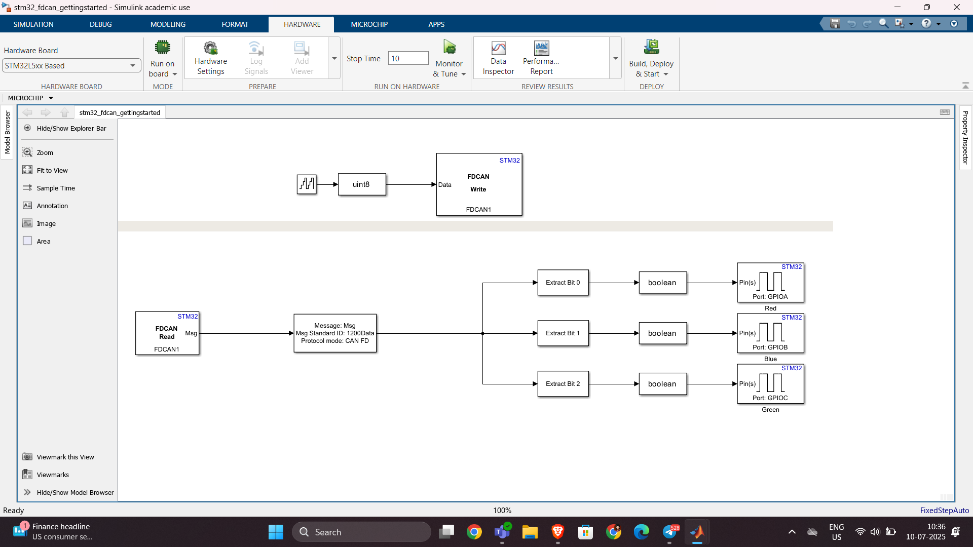
Hello,
I've successfully tested the Processor-in-the-Loop (PIL) workflow in Simulink using a TI F28069M LaunchPad, following the standard examples provided by MathWorks. The PIL block, code generation, and communication all worked without issues.
Now, I’d like to run a similar PIL setup using the Infineon TLE9879 EVALKIT (based on an ARM Cortex-M0), which is not officially supported by Simulink as a target.
I’m wondering if it’s possible to configure PIL manually or via custom workflows. For example:
- Can I create a custom PIL target using Embedded Coder?
- Would I need to port rtiostream manually for communication over UART?
- Could I somehow integrate with Keil µVision (which I use for TLE9879) to build and run the generated code?
- Is there a workaround to simulate PIL behavior using a non-supported board?
My setup:
- Simulink R2024b
- Infineon TLE9879 EVALKIT
- Keil µVision 5 + Infineon Config Wizard
- UART and JTAG interfaces available
The main purpose is to validate control algorithms and measure execution time, not to implement a full HIL system.
Has anyone attempted PIL with a custom or unsupported microcontroller before? Any tips or resources would be greatly appreciated. Thanks in advance!
Sto tentando inutilmente di salvare il valore dell'enegia che consumo ogni giorno nel field5 di questo canale: https://thingspeak.mathworks.com/channels/2851490 , ma inutilemte in quanto vengono visualizzati sempre e solo 2 dati anche se ho impostato days=30. Ho provato ad aumentare a 365 ma senza variazioni. Come mai?
Untapped Potential for Output-arguments Block
MATLAB has a very powerful feature in its arguments blocks. For example, the following code for a function (or method):
- clearly outlines all the possible inputs
- provides default values for each input
- will produce auto-complete suggestions while typing in the Editor (and Command Window in newer versions)
- checks each input against validation functions to enforce size, shape (e.g., column vs. row vector), type, and other options (e.g., being a member of a set)
function [out] = sample_fcn(in)
arguments(Input)
in.x (:, 1) = []
in.model_type (1, 1) string {mustBeMember(in.model_type, ...
["2-factor", "3-factor", "4-factor"])} = "2-factor"
in.number_of_terms (1, 1) {mustBeMember(in.number_of_terms, 1:5)} = 1
in.normalize_fit (1, 1) logical = false
end
% function logic ...
end
If you do not already use the arguments block for function (or method) inputs, I strongly suggest that you try it out.
The point of this post, though, is to suggest improvements for the output-arguments block, as it is not nearly as powerful as its input-arguments counterpart. I have included two function examples: the first can work in MATLAB while the second does not, as it includes suggestions for improvements. Commentary specific to each function is provided completely before the code. While this does necessitate navigating back and forth between functions and text, this provides for an easy comparison between the two functions which is my main goal.
Current Implementation
The input-arguments block for sample_fcn begins the function and has already been discussed. A simple output-arguments block is also included. I like to use a single output so that additional fields may be added at a later point. Using this approach simplifies future development, as the function signature, wherever it may be used, does not need to be changed. I can simply add another output field within the function and refer to that additional field wherever the function output is used.
Before beginning any logic, sample_fcn first assigns default values to four fields of out. This is a simple and concise way to ensure that the function will not error when returning early.
The function then performs two checks. The first is for an empty input (x) vector. If that is the case, nothing needs to be done, as the function simply returns early with the default output values that happen to apply to the inability to fit any data.
The second check is for edge cases for which input combinations do not work. In this case, the status is updated, but default values for all other output fields (which are already assigned) still apply, so no additional code is needed.
Then, the function performs the fit based on the specified model_type. Note that an otherwise case is not needed here, since the argument validation for model_type would not allow any other value.
At this point, the total_error is calculated and a check is then made to determine if it is valid. If not, the function again returns early with another specific status value.
Finally, the R^2 value is calculated and a fourth check is performed. If this one fails, another status value is assigned with an early return.
If the function has passed all the checks, then a set of assertions ensure that each of the output fields are valid. In this case, there are eight specific checks, two for each field.
If all of the assertions also pass, then the final (successful) status is assigned and the function returns normally.
function [out] = sample_fcn(in)
arguments(Input)
in.x (:, 1) = []
in.model_type (1, 1) string {mustBeMember(in.model_type, ...
["2-factor", "3-factor", "4-factor"])} = "2-factor"
in.number_of_terms (1, 1) {mustBeMember(in.number_of_terms, 1:5)} = 1
in.normalize_fit (1, 1) logical = false
end
arguments(Output)
out struct
end
%%
out.fit = [];
out.total_error = [];
out.R_squared = NaN;
out.status = "Fit not possible for supplied inputs.";
%%
if isempty(in.x)
return
end
%%
if ((in.model_type == "2-factor") && (in.number_of_terms == 5)) || ... % other possible logic
out.status = "Specified combination of model_type and number_of_terms is not supported.";
return
end
%%
switch in.model_type
case "2-factor"
out.fit = % code for 2-factor fit
case "3-factor"
out.fit = % code for 3-factor fit
case "4-factor"
out.fit = % code for 4-factor fit
end
%%
out.total_error = % calculation of error
if ~isfinite(out.total_error)
out.status = "The total_error could not be calculated.";
return
end
%%
out.R_squared = % calculation of R^2
if out.R_squared > 1
out.status = "The R^2 value is out of bounds.";
return
end
%%
assert(iscolumn(out.fit), "The fit vector is not a column vector.");
assert(size(out.fit) == size(in.x), "The fit vector is not the same size as the input x vector.");
assert(isscalar(out.total_error), "The total_error is not a scalar.");
assert(isfinite(out.total_error), "The total_error is not finite.");
assert(isscalar(out.R_squared), "The R^2 value is not a scalar.");
assert(isfinite(out.R_squared), "The R^2 value is not finite.");
assert(isscalar(out.status), "The status is not a scalar.");
assert(isstring(out.status), "The status is not a string.");
%%
out.status = "The fit was successful.";
end
Potential Implementation
The second function, sample_fcn_output_arguments, provides essentially the same functionality in about half the lines of code. It is also much clearer with respect to the output. As a reminder, this function structure does not currently work in MATLAB, but hopefully it will in the not-too-distant future.
This function uses the same input-arguments block, which is then followed by a comparable output-arguments block. The first unsupported feature here is the use of name-value pairs for outputs. I would much prefer to make these assignments here rather than immediately after the block as in the sample_fcn above, which necessitates four more lines of code.
The mustBeSameSize validation function that I use for fit does not exist, but I really think it should; I would use it a lot. In this case, it provides a very succinct way of ensuring that the function logic did not alter the size of the fit vector from what is expected.
The mustBeFinite validation function for out.total_error does not work here simply because of the limitation on name-value pairs; it does work for regular outputs.
Finally, the assignment of default values to output arguments is not supported.
The next three sections of sample_fcn_output_arguments match those of sample_fcn: check if x is empty, check input combinations, and perform fit logic. Following that, though, the functions diverge heavily, as you might expect. The two checks for total_error and R^2 are not necessary, as those are covered by the output-arguments block. While there is a slight difference, in that the specific status values I assigned in sample_fcn are not possible, I would much prefer to localize all these checks in the arguments block, as is already done for input arguments.
Furthermore, the entire section of eight assertions in sample_fcn is removed, as, again, that would be covered by the output-arguments block.
This function ends with the same status assignment. Again, this is not exactly the same as in sample_fcn, since any failed assertion would prevent that assignment. However, that would also halt execution, so it is a moot point.
function [out] = sample_fcn_output_arguments(in)
arguments(Input)
in.x (:, 1) = []
in.model_type (1, 1) string {mustBeMember(in.model_type, ...
["2-factor", "3-factor", "4-factor"])} = "2-factor"
in.number_of_terms (1, 1) {mustBeMember(in.number_of_terms, 1:5)} = 1
in.normalize_fit (1, 1) logical = false
end
arguments(Output)
out.fit (:, 1) {mustBeSameSize(out.fit, in.x)} = []
out.total_error (1, 1) {mustBeFinite(out.total_error)} = []
out.R_squared (1, 1) {mustBeLessThanOrEqual(out.R_squared, 1)} = NaN
out.status (1, 1) string = "Fit not possible for supplied inputs."
end
%%
if isempty(in.x)
return
end
%%
if ((in.model_type == "2-factor") && (in.number_of_terms == 5)) || ... % other possible logic
out.status = "Specified combination of model_type and number_of_terms is not supported.";
return
end
%%
switch in.model_type
case "2-factor"
out.fit = % code for 2-factor fit
case "3-factor"
out.fit = % code for 3-factor fit
case "4-factor"
out.fit = % code for 4-factor fit
end
%%
out.status = "The fit was successful.";
end
Final Thoughts
There is a significant amount of unrealized potential for the output-arguments block. Hopefully what I have provided is helpful for continued developments in this area.
What are your thoughts? How would you improve arguments blocks for outputs (or inputs)? If you do not already use them, I hope that you start to now.
Bom dia se alguém puder me ajudar, meu código abaixo, não estou conseguintdo conectar o meu Esp8266 ao ThingSpeak, o erro tá na conexão. Estou usando o MicroPython e NodeMCU na plataforma Pytohn o sistema operacional Ubuntu 20
# DHT11 -> ESP8266/ESP32
# 1(Vcc) -> 3v3
# 2(Data) -> GPIO12
# 4(Gnd) -> Gnd
import time, network, machine
from dht import DHT11
from machine import Pin
from umqtt.simple import MQTTClient
print("Iniciando...")
dht = DHT11(Pin(12, Pin.IN, Pin.PULL_UP))
estacao = network.WLAN(network.STA_IF)
estacao.active(True)
estacao.connect('xxxxxxx', 'xxxxxxxxx')
while estacao.isconnected() == False:
machine.idle()
print('Conexao realizada.')
print(estacao.ifconfig())
SERVIDOR = "mqtt.thingspeak.com"
CHANNEL_ID = "XXXXXXXXXXXXXXXXX"
WRITE_API_KEY = "XXXXXXXXXXXXXXXXXXXXX"
topico = "channels/" + CHANNEL_ID + "/publish/" + WRITE_API_KEY
cliente = MQTTClient("umqtt_client", SERVIDOR)
try:
while True:
dht.measure()
temp = dht.temperature()
umid = dht.humidity()
print('Temperatura: %3.1f °C' %temp)
print('Umidade: %3.1f %%' %umid)
conteudo = "field1=" + str(temp) + "&field2=" + str(umid)
print ('Conectando a ThingSpeak...')
cliente.connect()
cliente.publish(topico, conteudo)
cliente.disconnect()
print ('Envio realizado.')
time.sleep(600.0)
except KeyboardInterrupt:
estacao.disconnect()
estacao.active(False)
print("Fim.")
*****************************************************************************************************
No shell aparece como resposta:
MPY: soft reboot
Iniciando...
Conexao realizada.
('192.168.0.23', '255.255.255.0', '192.168.0.1', '8.8.8.8')
Temperatura: 29.0 °C
Umidade: 63.0 %
Conectando a ThingSpeak...
Traceback (most recent call last):
File "<stdin>", line 38, in <module>
File "umqtt/simple.py", line 67, in connect
OSError: -2
linha 38 é cliente.connect()
w = logspace(-1,3,100);
[m,p] = bode(tf(1,[1 1]),w);
size(m)
and therefore plotting requires an explicit squeeze (or rehape, or colon)
% semilogx(w,squeeze(db(m)))
Similarly, I'm using page* functions more regularly and am now generating 3D results whereas my old code would generate 2D. For example
x = [1;1];
theta = reshape(0:.1:2*pi,1,1,[]);
Z = [cos(theta), sin(theta);-sin(theta),cos(theta)];
y = pagemtimes(Z,x);
Now, plotting requires squeezing the inputs
% plot(squeeze(theta),squeeze(y))
Would there be any drawbacks to having plot, et. al., automagically apply squeeze to its inputs?
The ability to plot multiple signals on a plot and then use the plot browser to interactively control which ones are displayed has been one of the most useful features of the plotting tools and many of my scripts embed the command to open it after results analysis and plotting. It's been removed in 2025A with the comment that the Property Inspector provides the alternative. It doesn't. Having to go back into the menu to select the plot edit features to get to the Property Inspector (which doesn't provide an efficient alternative to the plot browser) has made the workflow very inefficient. Please bring it back a.s.a.p. !!!!
I want to use Simulink for model-based development of the TC3XX series development board, but I am not sure about the development process and toolchain? Is there a free toolchain available for me to use? Do you have a detailed development tutorial?
I have a pressure vs. time plot resulting from the input of an elastic wave, which I obtained from an Abaqus simulation. So, I have access to all the data. Now, I want to convert this time-domain graph into a frequency-domain graph using FFT in MATLAB.
I came across a code through ChatGPT, but I’m not fully confident in relying on it. Could anyone kindly clarify whether the formulas used for FFT in MATLAB are universal for all types of signals? Or is there a more effective and reliable method I should consider for this purpose?
Hi guys!
Im doing a project where i need to simulate a ship connected to the grid. I have a grid->converter AC-DC-AC -> dynamic load. My converter has to keep the voltage consistent and what changes is the current. Can somebody help me?
I like this problem by James and have solved it in several ways. A solution by Natalie impressed me and introduced me to a new function conv2. However, it occured to me that the numerous test for the problem only cover cases of square matrices. My original solutions, and Natalie's, did niot work on rectangular matrices. I have now produced a solution which works on rectangular matrices. Thanks for this thought provoking problem James.